| 18-02-2020 | François de Witte | treasuryXL |

Corporate Governance
Corporate Governance is a mechanism through which boards and directors can direct, monitor and supervise the conduct and operation of the corporation and its management in a way that ensures appropriate levels of authority, accountability, stewardship, leadership, direction and control.
The ultimate responsibility for Treasury management within an organization lies with the board of directors. Due to the practicalities and technical aspects involved in corporate treasury, the board typically delegates the daily management of risk to responsible individuals in each department. In the case of financial risks, many of these are delegated to the treasurer.
Whilst, due to its specific activities, the corporate treasurer needs to take a lot of actions and decisions independently, it is important that he does this within a framework and Governance. Quite a lot of corporates have formalized this in a “Corporate Treasury Policy”.
Corporate Treasury Policy
The Corporate Treasury Policy is the mechanisms by which the board, or risk management committee (RMC), can delegate financial decisions in a controlled manner. This document should be a summary of all the principles approved by the Board or the Financial Committee of the Board as a mandate of the Board to the treasurer (the Treasury Mandate).
The Corporate Treasury Policy is a framework document, which covers the following areas:
Organization of the Treasury Function
In most of the companies, the Corporate Treasury Reports to the CFO. The CFO is usually himself a Member of the Executive Committee, which itself reports directly to the Board of Directors. (Treasurer – CFO – Treasury Committee – Audit Committee – Board):
A policy should set out clearly which decisions are delegated to the treasurer and when the treasurer should refer a decision back to the board or other person within the organization. Within several corporate, the Board of Directors have delegated the decision process to dedicated committee, like the Risk Committee, and the Liquidity and Funding Committee.
Treasury Control Framework (including the Code of Conduct)
Procedures and controls to manage the risk should be put in place to provide an overall framework for decision-making by the treasury team.
Ideally, this should also include a code of conduct. The Corporate Treasurer should act as a Corporate Custodian. In other words, he is Protector of the company’s assets, and should act according to a strict Code of Conduct and Ethics. There exist examples of codes developed by professional organizations such as IGTA, ATEB, AFTE, ACT and ATEL.
Liquidity and funding
The board should be informed about funding possibilities to put currency, maturity, cost and equity/debt character into a wider context. The board should decide on the strategy but can delegate fund raising decisions and actions to treasury. However, I recommend that Treasury asks the final board approval for strategic decisions (e.g. major syndicated loans, bond issues, etc.).
The board should have an overall view on the liquidity risk of the company. The Board should also define the financial policy, covering the gearing and maturity issues, fixed and variable interest rate obligations, dividend policy and covenants.
Banking Relationship
Banks chosen by the treasurer must be able to meet the needs of the organization, both domestically and internationally. I recommend that the Board approves annually criteria for selecting the banks with whom it will work.
Risk Management
The Treasurer must identify the various risks to which the company is exposed, quantify the impact, and should inform the Board thereof. He should estimate the size of these exposure risks and their impact on the he overall operations and financial performance of the company, and make recommendations in these areas
The board must approve the hedging policy, the company’s foreign exchange, interest rate and commodity risk management policy and its attitude to risk. It should define which part of the risks must be hedged and the hedging horizon. I recommend that the Treasurer submits at regular intervals to the Board the list of authorized instruments, the amount per instrument and their term
Investment Policy – Counterparty Credit Risk
The board should approve the treasury’s Investment policy including the choice of instruments, the list of counterparties used + the maximum amount/counterparty & maturity. It is recommended that the Board provides guidelines and limits per instrument.
It is recommended that the Board approves the guidelines for fixing counterparty limits, and maximum exposure per counterparty.
Authorized instruments and Arrangements – Authorized Approvers
The Treasurer should make sure that the board must understands and approve the strategies and instruments used and sets guidelines for the appropriate limits for their use. These guidelines need to ensure that treasury has not sacrificed long-term flexibility or
survival for short-term gain, especially in view of the volatile financial market’s situation.
Treasury Operational Risk
The treasurer should make the Board aware of the operational risks to which the company is exposed. He should provide recommendations in this area. Furthermore, the treasurer should also submit recommendations to the board on the treasury organization and the ways to reduce the operational risks.
Monitoring
A Corporate Treasury Policy has only sense, if there is a regular follow up and control framework; Hence procedures and controls to manage the risk should be put in place to provide an overall framework for decision-making by the treasury team.
It is also important to provide to the Board a regular update on the way the treasurer complies with the policy. The policy should also be regularly reviewed.
Treasury must alert the board to external changes and internal strategic developments, which may have long-term implications for the organization and make proposals for managing them.
The policy needs also to be reviewed at regular intervals each “Policy” in function of the market and of other internal or external developments. I recommend having treasury on the Board’s agenda on a quarterly basis.
Conclusion
Treasury is not an island in the company. It is closely linked to the corporate governance. Hence it is important to define the right framework.
I recommend to corporates to put in place a treasury policy validated by the Board of Directors and reviewed regularly. It is important to update the Board at regular intervals about strategic topics, such as strategic financing topics and risk management.
The treasurer has also an important educational role, as he must be able to make complex treasury topics understandable for the board members.
Hence there must be a good interaction between the treasurer, the CFO and the Board is key, where the Treasurer is the linking pin.
 François de Witte
Founder & Senior Consultant at FDW Consult
Managing Director and CFO at SafeTrade Holding S.A.
treasuryXL ambassador


 There has been a significant rise in the value of the EUR in the last year compared to the USD. From a low of USD 1.05 around the end of February 2017, the EUR has climbed up to USD 1.25 – representing an increase of around 20 per cent. Analysts are talking about the price rising above USD 1.30 later this year. All very good from the EUR side, but what is causing the EUR to appear so strong and the USD so weak?
 Despite interest rate being very low for the last few years, general consensus is that rates will eventually rise – rates will become more normal. Rates are being held down by the actions of central banks with their quantitative easing. As QE is scaled backed and stopped this should allow rates to rise from their current low levels. The big question is – how high will rates rise? The Euro is not yet 20 years old and that means that whilst there is a lot of data, it does not require looking through 50 or 60 years of data to try and find the norm.
 Money Market outlook
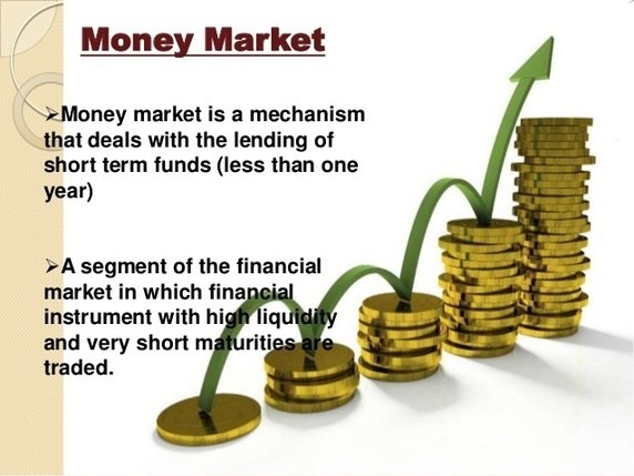
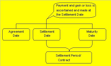
 where N is the notional of the contract, R is the fixed rate, r is the published -IBOR fixing rate and d is the decimalized day count fraction over which the value start and end dates of the -IBOR rate extend.

 You might visit this site, being a treasury professional with years of experience in the field. However you could also be a student or a businessman wanting to know more details on the subject, or a reader in general, eager to learn something new. The ‘Treasury for non-treasurers’ series is for readers who want to understand what treasury is all about. From our expert Victor Macrae we received another article on risk management, of which we thought that it adds some extra aspects to the earlier article on riskmanagement.