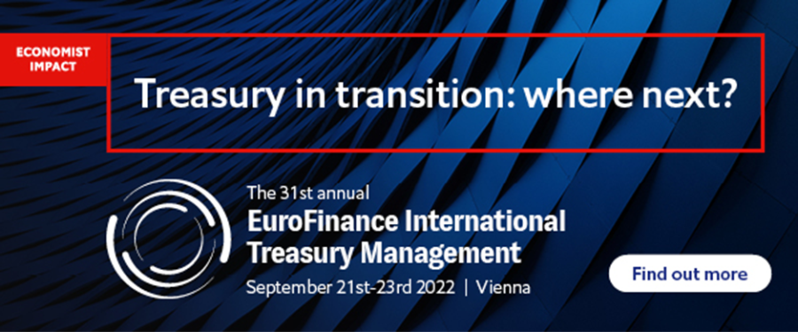
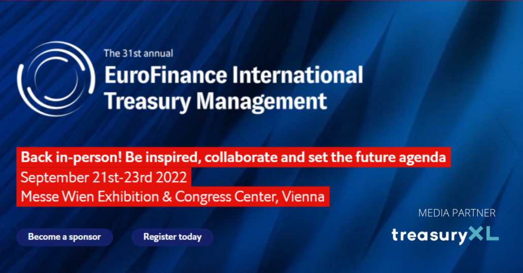
Basis Swap – how to convert your exposure

| 10-04-2018 | treasuryXL |

At the moment, there is a growing movement within interbank markets to replace all the existing interbank offer rates that are used to price a myriad of financial instruments. The motivation for this movement has been the revelation that these indices have been fraudulently priced by banks delivering inaccurate prices for the daily fixing. At the moment the markets are first looking at secured overnight lending indices – but these are not complimentary to all the existing instruments that regularly reference a longer tenor on an unsecured basis. These can lead to problems with the asset and liability management of a portfolio – not just for banks, but also for corporate clients.

So, what is a basis swap and how does it work?

A basis swap is an interest rate swap where both legs reference a floating rate – either in the same currency or on a cross currency. Examples would be a 3 month Euribor exposure against a 6 month Euribor exposure, or 3 month USD Libor versus 3 month GBP Libor. In a normal positive yield curve the interest rate for a longer tenor is higher than for the shorter period – 3 month USD Libor is 2.33746% and 6 month USD Libor is 2.47219%. There are 2 main reasons for the difference in price – the tenor is longer, therefore the risk of repayment is lengthened and the individual credit rating of the counterparty is also affected.

Before the financial crisis of 2008, basis swaps were traded, but not given much attention. Their primary function was for transforming the asset and liability management in the same currency. It was actively used in the cross currency market where a bank might raise long term funds in Japanese Yen, but needed to convert the proceeds into USD. Furthermore, the consensus at the time was that 1 master curve could be built to price all products – this used short dated deposits, 3 month interest rate futures and long date interest rate swaps to build the single curve.

This meant that a 6 month deposit was built on the basis of a 3 month deposit and a 3m v 6m FRA (Forward Rate Agreement) . In such an instance there would be no arbitrage possible and the market did not really look at the basis risk. But the basis risk was inherent and certain market players exploited this misconception – particularly banks that received fiduciary funding via Switzerland.

Today, there is far more awareness of the basis risk. 3 month Euribor is -0.329% and a 3v6m EUR FRA is -0.33/-0.31%. However the 6 month Euribor is 0.270% (we will leave you to do the calculation)

As a longer tenor has a higher interest rate (in normal market conditions) a basis swap referencing a 3 month versus 6 month payment would see the 3 month period being quoted as flat rate plus a premium, and the 6 month period being shown as a flat rate. A typical quotation for a 1 year EUR basis swap referencing a 3 month against 6 month Euribor would be priced around at about 5 -6 basis points premium. This means if you were to pay the shorter period of 3 months you would pay the base of 3 month Euribor plus 5-6 basis points every 3 months for 1 year, against receiving the 6 month Euribor flat every 6 months.

This product allows you to transform your position, but also gives insight into how the market sees the continuous 3 month and 6 month curves, together with their inherent basis risk.

An interest rate swap curve that references a 6 month floating leg, will normally be built from an interest rate swap curve built off a 3 month floating leg, with an adjustment for the 3m v 6m basis swap to reflect the higher price on a 6 month curve.


Davos, interest rates and secular stagnation

| 08-02-2018 | Lionel Pavey |


Two weeks ago there was the annual meeting of more than 2,000 politicians, business people, economists etc. at the World Economic Forum. For 4 days the most pressing and urgent topics facing the world were discussed. Sifting through all the speeches and press statements, I saw a lot of articles relating to a rather old theme of secular stagnation.

What is it?

It is a theory dating back to the 1930s stating that developed countries can suffer from a period of too small investment and too large savings. This can be the result not only of an economic recession but, more importantly, as the result of changes in the underlying demographics within a country. This would in turn imply that growth would be low to negligible within the economy. As growth slows down, so demand for investment would also slow down, leading to more savings etc.

Normal theory would demand a reduction in interest rates (the cost of money) leading to an increase in long term investments by companies, a comparative feeling of wealth amongst the people and a kick start to the economy.

Since the crisis of 2008, we have experienced an extended period of low interest rates and low inflation. The expected increase in investment, leading to improved production processes and new goods does not appear to have materialised. Furthermore, the effect that the crisis has had on individual people – job losses, house repossessions, insecurity – has made them reticent to indulge in large bouts of consumer spending.

Even with negative interest rates there has been no rush to invest in productivity. Instead funds are invested in financial assets – shares, bonds etc. Whilst offering goods returns, such investments do not add to potential economic productivity and growth in the industries that provide it.

Furthermore, when consumers tighten their belts – restricting spending and increasing savings – they are not actually directly providing funds for investment. Banks operate as intermediaries and extend credit – individual investors do not in the present system.

The economy is growing – GDP forecasts are all up among the major developed countries and inflation appears to be restrained. So have we broken the long existing chain of recognised monetary theory – could we see a prolonged period of steady growth, backed by low interest rates and low inflation?

At this stage of the proceedings an added element was thrown into the debates – demographics.

Europe is experiencing a period of shifting demographics. The long term replacement fertility rate is 2.1 children per woman. There has been a steep decline of this rate within Europe, with the rate in Germany being as low as 1.4 children. At the same time people are living longer, which means they are retired for longer. In 2006 there were 4 active workers for every retiree – by 2050 this could be down to only 2. The median age in Europe is expected to rise from 37 to 52 by 2050. EU studies have forecast that by 2050 there will be a reduction of 48 million in the working age population and an increase of 58 million in the retirees.

At the same time other studies suggest there will be a 14% decrease in working population against a 7% decrease in total population. All these projections are based on the current situation and that the trend continues.

If this was to continue, then there would be significant challenges for Europe. The expectation of governments to be able to finance the existing outstanding debt by increases in national GDP will stall. Increased burdens will be placed on the state to provide the necessary facilities to an ageing population whilst the pool of available workers is shrinking, leading to lower productivity per capita. Within the last 10 years the distribution of wealth has been skewed – there is more inequality with the super rich having proportionally even more of the total wealth than before the crisis.

New technology has the ability to change the existing concept of productivity. However, if this could be more than enough to offset the expected developments caused by an ageing population is unclear. It could mean that we are entering a prolonged period of low interest rates, low inflation and low growth. If so, all the economic models – even within companies – will need to be reappraised and a new long term policy initiated.

Lionel Pavey


Lionel Pavey

Cash Management and Treasury Specialist


The strength of the EUR or the weakness of the USD

| 07-02-2018 | treasuryXL |

There has been a significant rise in the value of the EUR in the last year compared to the USD. From a low of USD 1.05 around the end of February 2017, the EUR has climbed up to USD 1.25 – representing an increase of around 20 per cent. Analysts are talking about the price rising above USD 1.30 later this year. All very good from the EUR side, but what is causing the EUR to appear so strong and the USD so weak?

It is fairly well known that the Fed could be looking to increase interest rates in 2018 – consensus is for 3 small rises throughout 2018. As EUR interest rates are negative, initially one would expect a large movement out of EUR and into USD. But it looks as if the economies are aligned in the same way and any rise in USD rates could later be followed by a rise in EUR rates.

A lot will depend on the announcements by the ECB to taper off its QE programme. Long term EUR yields are rising in possible anticipation, but are still far behind USD yields. There is a 2 per cent yield pickup in 10 year USD treasuries over Germany who act as the benchmark for the EUR.

The posturing of the US administration and the words of President Trump appear to be having a negative impact on the value of the USD. Statements from Washington about a weaker USD being good for the US trade have impacted on the market. Trump has been very critical about trade relationships with other countries. The words being uttered by the administration are certainly having a reaction on the markets.

The Dow Jones saw a sell off on Friday – it lost more than 650 points. The job report that was published showed that the US had added 200,000 jobs in January but, despite this good news, fear is growing that this will put upward pressure on inflation, leading to further rises in treasury bond yields.

However, there are potential hazards in the future for the EUR. General elections in Italy are due to take place on the 4th March 2018. Current sentiment within Italy shows a growing negative appreciation of the EU. The trials and tribulations concerning Brexit could also seriously undermine the strength of the EUR.

Whilst it appears that the USD is weak at present, any adverse news from with the EU could lead to a swift reversal in fortunes. The underlying sentiment would imply a weaker dollar, but fundamental changes in economic policy on both sides of the Atlantic could lead to rapid changes in sentiment.


If you want more information please feel free to contact us via email [email protected]

What will be the new “normal” for interest rates?

| 23-01-2018 | Lionel Pavey |

Despite interest rate being very low for the last few years, general consensus is that rates will eventually rise – rates will become more normal. Rates are being held down by the actions of central banks with their quantitative easing. As QE is scaled backed and stopped this should allow rates to rise from their current low levels. The big question is – how high will rates rise? The Euro is not yet 20 years old and that means that whilst there is a lot of data, it does not require looking through 50 or 60 years of data to try and find the norm.

From a high of just over 5% in the summer of 2008, 10 year swap rates have fallen to a low of around 0.25% in the autumn of 2016 and are currently just under 1%. Historically, it has been usual to describe prices as moving back to around the average. However, having just under 20 years of data, it is possible to analyse the average fairly quickly.

The average rate for 10 year swaps for the last year is about 0.80%
The average rate for 10 year swaps for the last 2 years is about 0.70%
The average rate for 10 years swaps for the last 5 years is about 1.15%
The average rate for 10 year swap for the last 10 years is about 2.20%
And the average since 1999 when the Euro started is about 3.40%

The lowest rate was about 0.25% in 2016
The highest rate was about 6% in 2000

What is normal? From a personal point of view when I took out my first mortgage (back in the previous millennium) the advice I was given was that if long term fixed rates (10 years) were lower than 6.5% I should look to lock into that rate as the long term average was 7%. With every other property that I subsequently bought the long term fixed rates were lower than with my first mortgage. Currently mortgage rates for 10 year fixed are around 1.75%. Long term interest rates have been steadily falling for the last 30 – 35 years.

So, when we talk about rates eventually rising, we are still left with the problem that previous benchmarks – which were normal then – may not be applicable anymore.

A rate raise is absolute – the magnitude and its impact will be relative to our perception of the new “normal” benchmark.

Lionel Pavey


Lionel Pavey

Cash Management and Treasury Specialist


Forward Rate Agreement (FRA)

| 05-01-2018| Arnoud Doornbos |

Money Market outlook

At the press conference on 14 December 2017, the ECB announced that expectations for economic growth and inflation have been adjusted upwards. But despite optimistic growth, the ECB is not yet fully convinced of a continued upward trend in domestic price pressures. And thus Draghi: “An ample degree of monetary stimulus … is necessary for underlying inflation pressures to continue to build up.”

For this reason, the ECB will maintain the buying program at least until September 2018. And only then will an increase in policy rates come into the picture. Since the beginning of 2017, investors have seen the chance that the ECB will implement an increase in policy interest rates. This has not yet had an effect on the three-month Euribor rate. This has been stable at around -0.3% for the whole of 2017, and we expect that this will be the case in the vast majority of 2018 as well.

But markets will go up again for sure during time and borrowers need to prepare themselves for that moment. A good interest rate risk management can help to extent the pleasure of using favorable low interest rates for your company. Hedging your short term interest rate exposure with FRA’s could be a good idea. Good timing is essential.


Definition

A Forward Rate Agreement’s (FRA’s) effective description is a cash for difference derivative contract, between two parties, benchmarked against an interest rate index. That index is commonly an interbank offered rate (-IBOR) of specific tenor in different currencies, for example LIBOR in USD, GBP, EURIBOR in EUR or STIBOR in SEK. A FRA between two counterparties requires a fixed rate, notional amount, chosen interest rate index tenor and date to be completely specified.

FRAs are not loans, and do not constitute agreements to loan any amount of money on an unsecured basis to another party at any pre-agreed rate. Their nature as a IRD product creates only the effect of leverage and the ability to speculate, or hedge, interest rate risk exposure.


How it works

Many banks and large corporations will use FRAs to hedge future interest or exchange rate exposure. The buyer hedges against the risk of rising interest rates, while the seller hedges against the risk of falling interest rates. Other parties that use Forward Rate Agreements are speculators purely looking to make bets on future directional changes in interest rates.

In other words, a forward rate agreement (FRA) is a tailor-made, over-the-counter financial futures contract on short-term deposits. A FRA transaction is a contract between two parties to exchange payments on a deposit, called the Notional amount, to be determined on the basis of a short-term interest rate, referred to as the Reference rate, over a predetermined time period at a future date.

At maturity, no funds exchange hands; rather, the difference between the contracted interest rate and the market rate is exchanged. The buyer of the contract is paid if the published reference rate is above the fixed, contracted rate, and the buyer pays to the seller if the published reference rate is below the fixed, contracted rate. A company that seeks to hedge against a possible increase in interest rates would purchase FRAs, whereas a company that seeks an interest hedge against a possible decline of the rates would sell FRAs.


Valuation and Pricing

 The cash for difference value on a FRA, exchanged between the two parties, calculated from the perspective of having sold a FRA (which imitates receiving the fixed rate) is calculated as:

where N is the notional of the contract, R is the fixed rate, r is the published -IBOR fixing rate and d is the decimalized day count fraction over which the value start and end dates of the -IBOR rate extend.

For USD and EUR this follows an ACT/360 convention and GBP follows an ACT/365 convention. The cash amount is paid on the value start date applicable to the interest rate index (depending in which currency the FRA is traded, this is either immediately after or within two business days of the published -IBOR fixing rate).

For mark-to-market (MTM) purposes the net present value (PV) of an FRA can be determined by discounting the expected cash difference, for a forecast value r:

where vn is the discount factor of the payment date upon which the cash for difference is physically settled, which, in modern pricing theory, will be dependent upon which discount curve to apply based on the credit support annex (CSA) of the derivative contract.

Quotation and Market-Making

 FRA Descriptive Notation and Interpretation


How to interpret a quote for FRA?

[EUR 3×6  -0.321 / -0.301%p.a ] – means deposit interest starting 3 months from now for 3 month is -0.321% and borrowing interest rate starting 3 months from now for 3 month is -0.301%. Entering a “payer FRA” means paying the fixed rate (-0.321% p.a.) and receiving a floating 3-month rate, while entering a “receiver FRA” means paying the same floating rate and receiving a fixed rate (-0.321% p.a.).

Due to the current negative Money Market rates means receiving actually paying and the other way around.


Arnoud Doornbos 

Interim Treasury & Finance


2 most common financial risks faced by a company

| 16-6-2017 | Victor Macrae | treasuryXL |

You might visit this site, being a treasury professional with years of experience in the field. However you could also be a student or a businessman wanting to know more details on the subject, or a reader in general, eager to learn something new. The ‘Treasury for non-treasurers’ series is for readers who want to understand what treasury is all about. From our expert Victor Macrae we received another article on risk management, of which we thought that it adds some extra aspects to the earlier article on riskmanagement. 

An important task of a treasurer is to fully understand the financial risks that impact the firm. Two risks faced by most companies are interest rate risk and foreign exchange risk. Both risks can negatively impact the firm’s financial statements and can ultimately even lead to bankruptcy!

Interest rate risk

Interest rate risk originates from interest bearing liabilities. Most firms have loans. In the case the interest rate is variable, the interest paid varies according to an agreed market rate, such as Euribor or Libor. The risk is that the market rate will increase to a level where the firm is not able to pay its interest payments any more. In that case the firm is in default and theoretically the loan provider can request full loan redemption. In practice the loan provider is now in charge and will increase the margins on the loan as a result of the higher counterparty risk and also other charges such as fees of lawyers will be due. In order to mitigate interest rate risk a firm can use fixed rate loans or use variable rate loans in combination with interest rate derivatives such as interest rate swaps or options.

Foreign exchange risk

Foreign exchange risk occurs when a firm has subsidiaries abroad or when it transacts in a foreign currency. Suppose a firm with the euro as home currency sells products in Japanese Yen (JPY). Payment is due in three months’ time. If the JPY has weakened against the euro with 20% when the payment is due after three months, the revenues in euro are 20% lower. If the margin on the sales was 15%, then the negative foreign exchange rate change has led to a loss of 5%. Foreign exchange rate risk can be mitigated by various means, such a moving production to countries where the firm sell its products in order to match the currency of cash in- and outflows. Furthermore, derivatives such as forwards or options can be used to mitigate foreign exchange risk.

3 steps

The first step in managing interest rate risk and foreign exchange risk is to examine how the firm is exposed to these risks. The second step is to measure the impact of the volatility of interest and currency rates to which the firm is exposed on its financial statements. In the third step, if the effects are serious, the treasurer should consider which of the available options for risk mitigation best suits the firm.

Victor Macrae


Victor Macrae

Owner of Macrae Finance


Managing treasury risk: Interest rate risk (Part II)

|31-1-2017 | Lionel Pavey |


There are lots of discussions concerning risk, but let us start by trying to define what we mean by risk. In my first article of this series I wrote about risk managment and what the core criteria are for a solid risk management policy. Today I want to focus on interest rate risk. There are 4 types of interest rate risk.


Absolute Interest Rate Risk

Absolute interest rate risk occurs when we are exposed to directional changes in rates – either up or down. This is the main area of rate risk that gets monitored and analysed within a company as it is immediately visible and has a potential effect on profit.

Yield Curve Risk

Yield curve risk occurs from changes between short term rates and long term rates, together with changes in the spreads between the underlying periods. Under normal circumstances a yield curve would be upward sloping if viewed as a graph. The implication is that longer term rates are higher than short term rates because of the higher risk to the lender and less liquidity in the market for long dated transactions. Changes to the yield curve (steepening or flattening) can have an impact on decisions for investment and borrowings, leading to changes in profit.

Refunding or Reinvestment Risk

Refunding or reinvestment risk occurs when borrowings or investments mature at a time when interest rates are not favourable. Borrowings or investments are rolled over at rates that had not been forecast leading to a potential loss on projects or investments.

Embedded Options Risk

Embedded options are provisions in securities that cannot be traded separately from the security and grant rights to either the issuer or the holder that can introduce additional risk. Benefits for the issuer can include a call option, a right to repay before maturity without incurring a penalty, an interest rate cap. Benefits for the holder can include a put option, a conversion right via convertible bonds, an interest rate floor.


An attempt can be made to calculate the interest rate risk on either a complete portfolio or on individual borrowings or investment. This is done by comparing the stated interest rate to the actual or projected interest rate. Methods include:

  1. Mark to market
  2. Parallel shift in the whole yield curve
  3. Tailor-made shift in the whole yield curve
  4. Duration, DV01, Convexity
  5. Value at Risk (VaR)

These are all forms of quantitative analysis and well recognized. Personally I am of the opinion that VaR is not a very good method for interest rates. Interest rates do not display normal Gaussian distribution – they do not resemble a normal bell curve. Interest rate distribution curves display fat tails compared to normal statistical models.

Financial products that are commonly used to manage interest rate risk include FRAs, Futures, Caps, Floors, Collars, Options, Interest Rate Swaps and Swaptions.

Lionel Pavey


Lionel Pavey

Cash Management and Treasury Specialist


More articles from this author:

Safety of Payments

The treasurer and data

The impact of negative interest rates

How long can interest rates stay so low?


Managing interest rate and liquidity risk

| 06-09-2016 | Rob Söentken |

skyscrapertxl


Funding is one of the key focus areas of a treasurer. There are numerous dimensions to funding:
1. Assessing amount and timing of cashflows
2. Arranging access to funding
3. Developing and implementing hedging policy
4. Optimizing funding cost and risk

Assessing amount and timing of cashflows

Assessing the amount and timing of cashflows is a continuous process. Because needs can change both in short and long term.

Arranging access to funding

Matching funding needs with supply from financial institutions is also a continuous process. The typical approach would be to match tenors, but immediate access to cash is critical for the survival of any entity. It could be considered to arrange longer term financing, even for short term (revolving) funding needs. The downside is that long term access is more expensive than short term access. This may be acceptable, but if the spread between borrowing and lending excess cash is too wide, it will become very unattractive to borrow for long tenors.

Developing and implementing hedging policy

To ensure the treasurer works within the boundaries of his mandate, he has to develop a hedging policy which must be documented (‘on paper’) and approved by his management. The document should describe the whole area of funding, to ensure both the creation and hedging of risks are described.

Optimizing funding cost and risk

The main focus drifts towards reducing funding cost. The funding market typically has a steep cost curve, meaning that rates are higher for longer tenors. This results from a steep ‘risk free’ curve and / or from a steep ‘credit spread’ curve. Which often brings entities to borrow for the cheapest tenor possible, being monthly, weekly or even overnight funding. Funding for very short tenors creates the considerable risk that can cause a company to run into a liquidity crisis, in case access to funding disappears. How to deal with this dilemma?

The best approach is to define a number of scenarios to assess the impact of combinations of financing and hedging on funding and risk. A base scenario could be to finance all funding needs using overnight loans. In case of liquidity problems, what would be the impact on the funding rates? Another scenario would be using quarterly funding or yearly rollover funding, potentially combined with:

  • money market futures
  • interest rate swaps
  • caps / floors
  • bond futures or even
  • credit derivatives

What are the incremental funding cost? What are incremental operational expenses of running various products? Can the entity deal with managing margin requirements? Is the entity aware of the basis risks involved when using credit derivatives, which are fairly complex products?

Rob Soentken


Rob Söentken

Ex-derivatives trader


The impact of negative interest rates

01-08-2016 | Lionel Pavey |

rating


Articles in the press state that large commercial banks are considering charging their corporate clients negative interest rates on credit balances on their bank accounts. This presents us with certain problems – how will clients react?

Withdraw money – known as stuffing money under the mattress. This would present huge security issues on where the money could be safely kept, potential theft etc. Holding cash would give a return equal to zero, which would be greater than depositing it at a bank.

Hoarding – by withdrawing money from the banking system, banks themselves would have less money to lend and would force them to reduce their balance sheets. Conversely the idea would be that people would spend more money rather than save and, therefore, boost the economy. Would it work? We are seeing negative yields on high quality government bonds, for a variety of reasons, yet it appears that negative rates have not boosted spending or investment. The loosening of monetary policy does not appear to have removed market fears.

Disintermediation – banks fulfill a role as intermediar/middleman in the supply chain of finance. If money is withdrawn from the banking system it would be even harder for banks to provide finance to lenders. How could lenders then obtain the funding they require? Virtual marketplaces could be envisaged but there are so many security and safeguard issues that would need to be addressed before this could take place. Most companies can not borrow from capital markets – they rely on banks to provide their funding. Reductions in government bond yields to below zero do not lead to more funding being given to companies.

Worst case scenarios – companies will invest in technologies that are capital intensive leading, eventually, to a fall in the demand for labour. Pensioners who are dependent on interest income will be forced to reduce their consumption leading to a fall in demand. With safe yields being negative the search for yield could lead investors into riskier assets than they would normally consider.

A stamp on physical cash – this is an idea more than 100 years old proposed by Gesell to stop hoarding of cash. Bank notes would need to receive a stamp every month to be considered valid cash. These stamps would have to be purchased (a form of negative interest) and their purpose would be to erode the principle that money is a store of value and could be better used by being actively invested in the economy.

This all sounds very pessimistic, but there are potential gains from negative interest rates for companies.

It would encourage companies to pay their creditors more quickly and, in the process, receive discounts on their purchases outstanding if they pay early. Furthermore it would enable companies to truly examine their whole supply chain across all departments within a company and create a better understanding of the workflow processes concerning cash receipts and disbursements.

For those who like a more rogue approach, you could actually overpay your creditors and ask for a credit note. Now your creditor is funding your negative interest rate and if true economic theory principles are maintained – a fall in prices should follow negative interest rates – then, not only you would have handed over your negative interest rate exposure but you would also benefit from falling prices in the future on the outstanding credit notes with your creditors allowing you to make a relative saving on the future purchase price.

It is clear that steering interest rates will not sort out the economy – other steps outside of monetary policy will have to be taken to restore faith in the economy. But which steps will that be?


Lionel Pavey


Lionel Pavey

Cash Management and Treasury Specialist


Zero Coupon Yields and implied Forward Yields

| 13-06-2016 | Lionel Pavey |


Having constructed our 20 year yield curve with both observable data and discovered data in my previous article,we are now in possession of 3 sets of data:

  1. Spot par rates
  2. Spot zero coupon rates
  3. Discounted Cash Flow factors (DCF)

The most important of these, for calculation purposes, is DCF.

Present Value

The discounted present value of a future cash flow can be calculated by dividing the future value by the DCF. It therefore follows that a series of future cash flows can also be discounted to a single net present value.

Implied Forward Rates

The original yield curve showed annual spot rates for a period of 20 years. Using DCF it is possible to construct similar curves but with forward start dates – a curve starting in 1 year, 2 years, 3 years etc. When building these curves the “implied” forward rate will actually be a zero coupon rate and not a par rate. Converting the zero rates to par rates can be achieved by using Excel Solver – a very useful tool but great care must be taken as Solver gives an answer but shows no formula.

So, how do we calculate an implied forward rate?

Let us assume that we wished to find a rate with a duration of 4 years, starting 5 years forward.
To achieve that, we need both the 5 year DCF and the 9 year DCF

The previous constructed curve yields the following values –

5Y DCF                    =               0.9464924176

9Y DCF                    =               0.8508986778

((.9464924176/.8508986778)^(1/4)-1)*100     =  2.6975% implied 4 year rate starting in 5 years

As stated, this is the implied zero coupon rate – the implied par rate is 2.6887%

All forward rates are purely implied rates – a true quoted rate would always be different for various reasons –

  1. Spread between bid and offer
  2. Yield curve constructed with specific data
  3. Sentiment of the trader
  4. Possible exposure already in the banks’ books

Here is a small snapshot of both implied rates and par rates built with the original curve.

parrates complied rates

When I discussed building the original yield curve, different ways of interpolation were tried. I would now like to show how small differences in yields in a spot curve can lead to significant differences in a forward curve.

Let us look at a duration of 5 years starting 10 years in the future and compare the linear interpolation with the smooth adjusted curve. Assume that the instrument to be priced is a linear instrument – equal repayments of principal every year.

I have built both curves using the same layout and formulae throughout with the exception of the input rates in the missing periods.

The linear rate is 3.276%; the smooth adjusted rate is 3.416% – a difference of 14 basis points or about 4% of the smooth rate. In a market where the normal bid/offer spread is about 3 or 4 basis point, this represents a significant difference/anomaly.

I regularly hear people say that when they need to purchase a financial instrument that they get at least 2 quotes – this is all very well but does not stop a treasurer from first ascertaining what the correct price should be before getting a quote. If banks know that, as a treasurer, you can not calculate the theoretical price this allows them to move the price away from the implied to a price that is more advantageous to them and their trading book! A dedicated financial data vendor system can make life easier, but it is not impossible to calculate a price without these resources!


Next – Spreads; their use and the hidden extra costs

First two articles on building a yield curve:
1. Yield Curves (term structure of interest rates) – filling in the blanks
2. Yield Curves (term structure of interest rates) – filling in the blanks part II


Lionel Pavey


Lionel Pavey

Treasurer