Tag Archive for: interest rate swaps

Saving on FX deals? Often neglected but potentially a “pot of gold”

| 21-8-2017 | Patrick Kunz |


Doing business internationally often means dealing with foreign currency (FX). This poses a risk as the exchange rate changes daily, basically every second. To mitigate this risk a company can hedge the position via FX deals (discussed in a previous article). But what are the costs of those deals to companies?


FX deals

FX is traded on exchanges where only authorized parties have access to. This can be brokers or banks, the so called market makers. They can take your fx position for a give rate and they try to find a counterparty for the deal who is willing to take the opposite trade. For this effort (and risk as they might not be able to directly match the position) they ask a provision. This is the bid-ask spread; the spread between rate for buying and rate for selling the currency. The fx (mid) rate is determined by supply and demand.

The spread depends on several things:

  • Market liquidity; how many people are buying and selling and with what volume
  • Market timing; is the market open for that currency
  • Restrictions: some currencies have restrictions

For a company to trade FX they need an account with a party that has access to fx market makers. This is often a bank. This bank will take another bite out of the spread for their profit (and maybe risk as they might take the position on their books). The spread the bank will charge depends on how many deals and how much volume you will be doing. Sometimes it is an obligation to trade with the bank from a financing arrangement. For the big currencies for big clients the spread can be as low as 2-3 pips (0,0002/0,0003).

Trading FX seems to be without costs as the bank charges no fees. However, those fees are put into the fx rate. When doing spot deals it is easy to calculate them, it’s the difference between the traded rate and the then actual market spot mid rate. When doing forward deals or trading illiquid currencies it is harder to determine the spread. Always try to get to know the spread you are paying. The spread is basically the costs of the fx deal (for forward deals there is an interest component).

It therefore makes sense to always compare your FX rates and get quotes from several banks. Trading with a broker sometimes can be cheaper as one party in the process is eliminated. Savings can be up to 5% per deal (for exotic currencies), for the bigger currencies an average saving of 1% is possible. If you do several million worth on FX deals a year this is a big money saver.

Pecunia Treasury & Finance b.v. has an online fx trading platform backed by one of the biggest worldwide fx broker.

Patrick Kunz

Treasury, Finance & Risk Consultant/ Owner Pecunia Treasury & Finance BV


Basel III and the impact on cost of hedging

| 30-3-2017 | Arnoud Doornbos | Treasury Services |

Corporates will save hedging costs and administrative costs significantly if they shift their hedging activities to exchanges such as CME (Chicago Mercantile Exchange).
In the summer of 2007 a large number of defaults on U.S. mortgage loans did arise. The banks were hit hard by the global domino effect that resulted. A major financial crisis which was followed by an economic crisis led to a revision of the capital requirements of Basel I and Basel II.

New Basel III

The core of Basel III is that many banks have to hold more capital and liquidity to their outstanding investments than they used to in the past. The rules are implemented as from 2013 and should eventually be fully effective in 2019.

Basel III will be a huge challenge for banks in the coming years. The impact on the pricing of financial products and transactions between banks and their clients will be significant.
Since July 2008, the Basel Committee for Banking Supervision has been working on Basel III for all banks worldwide. The European Commission has introduced three Capital Requirements Directives which contains concrete actions and requirements in terms of risk, capital and liquidity management within a bank. The new requirements, part of Basel III, aim to improve the quality and level of capital reserves of banks.

The capital requirements of certain products have increased and banks are encouraged to create additional capital buffers during good economic times so that they are better positioned to absorb losses during periods of economic stress.

Impact of Basel III on liquidity management

Besides sharpening the capital requirements Basel III has a major impact on liquidity management. The new liquidity standards are based on a stress test. In addition Basel III also introduces new long-term liquidity standards that reduce the mismatch between the maturities of assets and liabilities.
Banks will have to increase their reserves sharply in the coming years. Previously, banks only had to keep 2 % capital to their outstanding investments. Now with Basel III this capital requirement has been increased to 7 % (4.5 % hard buffer and an additional 2.5 % margin in bad times) . As a result banks will probably not distribute their profits in the coming years but will add to their capital buffers. Furthermore many banks will have to issue new shares in order to attract extra money in order to meet the new demands.

Counterparty risk

Within Basel III it has been determined that capital must be held for the credit risk on a counterparty a bank is exposed to in OTC derivatives or equity financing transactions. In addition, market participants are encouraged to take one central counterparty (clearing houses) for OTC derivatives. Any time a bank takes a risk against another party the probability of default exists. To offset this concern, and to support on-going stability within the interbank market, banks have long emphasized the importance of measuring and managing counterparty risk. Now banks have becomes noticeably less comfortable trading with other counterparties including other banks.

The recent deterioration in credit ratings that has hit many U.S. and European banks has led to a heightened sensitivity over counterparty risk. These apprehensions may not be voiced directly, but they become evident when front office trades that would have cleared in the past, no longer do because credit lines have been reduced. There is increasing focus on limiting exposures, even among global banks. And that is starting to affect the way we do business.
CVA (Credit Valuations Adjustment) desks have grown in popularity, as banks seek more effective ways to manage and aggregate counterparty credit risk.
The market has changed now in terms of how counterparty credit risk was calculated. Now, no client is assumed to be truly risk free. Different prices are now expected for different clients on that same interest rate swap, depending on variables including the client’s rating and the overall direction of existing trades between both parties.
On all new interest rate, FX, equity, or credit derivatives, CVA desks price the marginal counterparty risk for inclusion into the overall price charged to the client. CVA is a highly complex calculation.

CVA looks at default through the spread of the counterparty. A swap facing a single B credit that trades at 1200 in CDS is going to be charged a lot more than the same swap facing a AA counterparty. The CDS spread is normally a core input of CVA pricing.

What we see in practice is that in the manual process, the CVA desk team of a bank often passes along suggestions to the salesperson for improving the credit risk in a trade and enabling the sales person to offer the trade at a lower credit price. Examples of that would include improving the collateral agreement with a client, or inserting a break clause.
In the traditional CVA approach, a bank accepts a new trade, takes a fee and uses that fee to buy good hedges for all the risks in that trade. These hedges should eliminate all of the bank’s risk, but this is not necessarily the case once Basel III is taken into account.

Basel III does not recognize all types of hedges that the bank might want to use. Therefore the regulatory capital for certain trades will not be zero, even if the bank has used the full CVA fee to hedge all its risks.
The first impact Basel III has on CVA desks is on pricing. Pre-deal pricing needs to be reviewed to ensure the costs of imposed regulatory capital are covered. If not, additional pricing may need to be added. And the decision on which risks are efficient to hedge also becomes affected not just by strategic or business reasons, but also by the regulatory capital impact.
As part of Basel III’s updated regulatory capital guidelines, a new element has been added: V@R on CVA. Regulators have specified very precisely how the underlying CVA must be calculated for this charge. Banks will therefore need to decide whether to adjust their pricing and balance sheet CVA to match the Basel III rules, or to use different CVA calculations for pricing and regulatory purposes.

EMIR / Dodd-Frank

The Dodd-Frank / EMIR financial reform bill gives a new set of derivatives rules that either will clean up the market or send the world spiraling off the deep end. The truth is probably somewhere in between. The crux of the derivatives regulation is the requirements that standardized swaps be centrally cleared and traded on a Swap Execution Facility, or SEF. This moves derivatives from bilateral agreements between bank and client to centrally cleared products where credit risk is no longer bank-held, but is centralized in a clearinghouse where daily margin is managed. Once clearing is in place, customers no longer are locked into a single dealer, long and short positions can be netted, and SEFs can begin to match buyers and sellers without having to worry about the credit lines of each counterparty or dealer.

This will begin the migration of the derivatives business from a principal-based OTC market toward an agency-based bid/offer SEF market.

Treasury Services’ analysis:

  • Hedging is penalized decreasing the liquidity in the markets leading to increased costs to hedge financial risks for corporations. This is further emphasized by the penalization of the interbank markets through requirement of more capital, and additional constraints on liquidity on interbank transactions.
  • There will also be an increase in administration costs for corporates costs due to EMIR.
  • Corporate credit by banks is penalized: More capital is required in general. For back-up facilities on commercial paper programs it is required that banks will have to have 100% of liquid assets whilst these facilities are fully undrawn. The cost of carry will obviously be invoiced to the client. The ability of the bank to borrow long term will determine the availability of back-up facilities.
  • Restrictions in maturity mismatch (including for repayments) are introduced. This may mean that the risk of borrowing short term to finance long term investments will be transferred to the corporate sector.

The advantages of the OTC market compared to exchanges has become questionable. High cost savings can be achieved by shifting your hedging activities to exchanges such as Chicago Mercantile Exchange (CME).
Shifting hedging activities to an exchange such as CME requires changes in your risk management function. This supplies the possibility to bring the cost of hedging back in your control.


Arnoud Doornbos

Associate Partner

Uniform Herstelkader Rentederivaten MKB

| 21-2-2017 | Simon Knappstein |


Op 19 december van vorig jaar is het definitieve herstelkader rentederivaten gepubliceerd door de Derivatencommissie. Dit is een update van de versie die al in juli van 2016 werd gepubliceerd. De update is inhoudelijk onveranderd maar bevat een aantal toelichtingen en bijlagen om de werking van het herstelkader te verduidelijken.
De opdracht om dit herstelkader op te stellen is door de Minister van Financiën in maart 2016 gegeven. Alle Nederlandse banken hebben zich aan dit herstelkader gecommitteerd.

Tegelijk met deze publicatie heeft de Derivatencommissie ook een informatieve brochure uitgegeven.  Banken zullen deze gaan opnemen in hun brieven die ze naar klanten met renteswaps gaan sturen. Hierin wordt op hoofdlijnen de werking van de compensatieregeling uitgelegd.
Eerst wordt het toepassingsbereik geschetst, voor wie geldt dit herstelkader?
Dit herstelkader is van toepassing op niet-professionele partijen die niet aan deskundigheids-eisen voldoen. Dat betekent in de praktijk dat het met name gaat om MKB-ondernemingen en particulieren. Verder gelden er voorwaarden met betrekking tot de looptijd van de rentederivaten. (Een interessante ontwikkeling is dat het gerechtshof in Den Haag gisteren geoordeeld heeft dat een groot bedrijf toch recht heeft op schadevergoeding voor renteswaps die de bank heeft verkocht, als vooraf duidelijk was dat het bedrijf geen speciale kennis had over dit soort financiële instrumenten.)

Vier stappen

Vervolgens zijn er vier stappen gedefinieerd om de hoogte van de compensatie te bepalen.

In stap 1 worden gestructureerde, complexe derivaten door de banken aangepast naar een renteswap, een rentecap of een rentecollar. Het verschil in netto cashflows wordt in deze stap gecompenseerd.

In stap 2 worden alle verschillen tussen het derivaat en de onderliggende financiering aangepast. Denk hierbij aan een overhedge in omvang, een overhedge in looptijd of afwijkingen in referentierente. Ook hier worden de verschillen in netto cashflows gecompenseerd.

In stap 3 bieden de banken een coulancevergoeding aan. Deze vergoeding bedraagt maximaal 20% van de rente die per saldo onder een renteswap dan wel rentecollar aan de bank is betaald en naar verwachting nog zal worden betaald. Deze vergoeding is gemaximeerd op €100.000,-. Mijn ervaring is dat met een looptijd van 10 jaar en een hoofdsom van €2,0 mio a €2,5 mio dat maximum wel bereikt wordt.

In stap 4 vergoeden banken onverwachte verhogingen van renteopslagen op financiering(en) die door een renteswap worden afgedekt.
De banken verwachten dat zij in de loop van 2017 hun klanten kunnen informeren met concrete compensatievoorstellen. De exacte timing zal per bank verschillen. Als de bank een voorstel heeft gedaan, kan de klant beslissen of hij van het voorstel gebruik maakt. Bij acceptatie van het voorstel, verleent hij finale kwijting aan de bank.

Toezichthouder AFM gaat er op toezien dat de banken en de externe beoordelaars dit proces zorgvuldig en volledig uitvoeren.

Als u meer wilt weten over dit herstelkader kunt u mij mailen op [email protected]

Simon Knappstein - editor treasuryXL


Simon Knappstein

Owner of FX Prospect


Managing treasury risk: Commodity Risk (Part IV)

| 14-2-2017 | Lionel Pavey |

There are lots of discussions concerning risk, but let us start by trying to define what we mean by risk. In my fourth article I will write about commodity risk, what the strategies around commodities are and how to build a commodity risk framework. More information about my first three articles can be found at the end of today’s article.

Commodity Risk

Commodity risk occurs due to changes in price, quantity, quality and politics with regard to the underlying commodities. This can refer to both the commodity as a whole and an input component of a finished good. Commodity risk usually refers to the risk in a physical product, but also occurs in products like electricity. It can affect producers, suppliers and buyers.

Traditionally, commodity price risk was managed by the purchasing department. Here the emphasis was placed on the price – the lower the price, the better. But price is only one component of commodity risk. Price changes can either be observed directly in the commodity or indirectly when the commodity is an input in the finished product.
Availability, especially of energy, is crucial for any company to be able to undertake operations. Combining commodity risk over both Treasury and Purchasing allows these 2 departments to work closer and build a better understanding of the risks involved. It also allows for a comprehensive view of the whole supply chain within a company. A product like electricity is dependent on the input source of production – gas, petroleum, coal, wind, climate – as well as the price and supply of electricity itself.

There are many factors that can determine commodities prices – supply and demand, production capacity, storage, transport. As such it is not as easy to design the risk management model as it is for financial products.

 General strategies that can be implemented

  1. Acceptance
  2. Avoidance
  3. Contract hedging
  4. Correlated hedging

Acceptance
Acceptance would mean that the risk exposure would be unchanged. The company would then absorb all price increases and attempt to pass the increase on when selling the finished product.

Avoidance
Avoidance and/or minimizing means substituting or decreasing the use of certain input components.

Contract hedging
Contract hedging means using financial products related to the commodity, such as options and futures as well as swapping price agreements.

Correlated hedging
Correlated hedging means examining the exposure of a commodity – the price of crude oil is always quoted in USD – and taking a hedge in the USD as opposed to the crude oil itself. The 2 products are correlated to a certain extent, though not fully.

Commodity risk framework

Commodity price speculation – most contracts are settled by physical delivery – affects the market more than price speculation in currency markets.
To build a commodity risk framework, attention needs to given to the following:

  1. Identify the risks
  2. Measure the exposure
  3. Identify hedging products
  4. Examine the market
  5. Delegate the responsibility factors within the organization
  6. Involve management and the Board of Directors
  7. Perform analytics on identified positions
  8. Consider the accounting issues
  9. Create a team
  10. Are there system requirements needed

Problems can arise because of the following:

  1. Relevant information is dispersed throughout the company
  2. Management may not be aligned to the programme
  3. Quantifying exposure can be difficult
  4. There is no natural hedge for the exposure
  5. Design of reports and KPI’s can be complex

It requires an integrated commitment from diverse departments and management to understand and implement a robust, concise policy – but this should not be a hindrance to running the policy.

Lionel Pavey


Lionel Pavey

Cash Management and Treasury Specialist 


More articles of this series:

Managing treasury risk: Risk management

Managing treasury risk: Interest rate risk 

Managing treasury risk: Foreign exchange risk


Managing Treasury Risk – Foreign Exchange Risk (Part III)

| 7-2-2017 | Lionel Pavey |


There are lots of discussions concerning risk, but let us start by trying to define what we mean by risk. In my third article I will focus on foreign exchange risk. This risk has to be taken into consideration when a financial commitment is denominated in a currency other than the base currency of a company.
There are 4 types of foreign exchange risk.

Transaction Risk

Transaction risk occurs when future cash flows are denominated in other currencies. This refers to both payables and receivables.  Adverse changes in foreign exchange prices can lead to a fall in profit, or even a loss.

Translation Risk

Translation risk occurs when accounting translation for asset and liabilities in financial statements are reported. When consolidating from an operating currency into a reporting currency (overseas offices etc.) the value of assets, liabilities and profits are translated back to the reporting currency. Translation risk does not affect a company’s cash flows, but adverse changes can affect a company’s earnings and value.

Economic Risk

Economic risk occurs when changes in foreign exchange rates can leave a company at a disadvantage in comparison to competitors. This can affect competitive advantage and market share. Future cash flows from investments are also exposed to economic risk.

Contingent Risk

Contingent risk occurs when potential future work is expressed in a foreign currency. An example would be taking part in a tender for work in another country where the pricing is also in a foreign currency. If a company won a large foreign tender, which results in an immediate down payment being received, the value of that money would be subject to transaction risk. There is a timeframe between submitting a tender and knowing if the tender has been won, where a company has contingent exposure.

Identifying Foreign Exchange Risk

  1. What risk does a company face and how can it be measured
  2. What hedging or rate management policy should a company use
  3. What financial product, available in the market, should be best used
  4. Does the risk relate to operational cash flows or financial cash flows

Initially we need to ascertain what we think future FX rates will be. Methods that can be used include the Forward Rate Parity, the International Fisher Effect which also includes expected inflation, forecasts provider by banks and international forums, along with VaR. Model analysis can be provided, among others, via fundamental factors, technical analysis, and political analysis.

Different FX rates can then be used to simulate the effects on cash transactions when converted back into the base currency. This will provide different results that will allow a company to determine what level of risk it is prepared to accept. Finally a decision must be taken as to whether the company wishes to hedge its exposure or not. Before the advent of the Euro, both the Netherlands and Germany  were members of the Exchange Rate Mechanism (ERM). This meant there was agreed band within which the spot rate could move around an agreed central point – this was NLG 112.673 equal to DEM 100.00 with a bandwidth of +- 2.25%. For some companies, this tight band meant that they took the decision not to hedge any exposure between DEM and NLG.

Financial products that are commonly used to manage foreign exchange risk include Forward Exchange contracts, Futures, Caps, Floors, Collars, Options, Currency Swaps and Money Market hedging.

Lionel Pavey


Lionel Pavey

Cash Management and Treasury Specialist


More articles of this series:

Managing treasury risk: Risk management

Managing treasury risk: Interest rate risk 

Managing treasury risk: Interest rate risk (Part II)

|31-1-2017 | Lionel Pavey |


There are lots of discussions concerning risk, but let us start by trying to define what we mean by risk. In my first article of this series I wrote about risk managment and what the core criteria are for a solid risk management policy. Today I want to focus on interest rate risk. There are 4 types of interest rate risk.


Absolute Interest Rate Risk

Absolute interest rate risk occurs when we are exposed to directional changes in rates – either up or down. This is the main area of rate risk that gets monitored and analysed within a company as it is immediately visible and has a potential effect on profit.

Yield Curve Risk

Yield curve risk occurs from changes between short term rates and long term rates, together with changes in the spreads between the underlying periods. Under normal circumstances a yield curve would be upward sloping if viewed as a graph. The implication is that longer term rates are higher than short term rates because of the higher risk to the lender and less liquidity in the market for long dated transactions. Changes to the yield curve (steepening or flattening) can have an impact on decisions for investment and borrowings, leading to changes in profit.

Refunding or Reinvestment Risk

Refunding or reinvestment risk occurs when borrowings or investments mature at a time when interest rates are not favourable. Borrowings or investments are rolled over at rates that had not been forecast leading to a potential loss on projects or investments.

Embedded Options Risk

Embedded options are provisions in securities that cannot be traded separately from the security and grant rights to either the issuer or the holder that can introduce additional risk. Benefits for the issuer can include a call option, a right to repay before maturity without incurring a penalty, an interest rate cap. Benefits for the holder can include a put option, a conversion right via convertible bonds, an interest rate floor.


An attempt can be made to calculate the interest rate risk on either a complete portfolio or on individual borrowings or investment. This is done by comparing the stated interest rate to the actual or projected interest rate. Methods include:

  1. Mark to market
  2. Parallel shift in the whole yield curve
  3. Tailor-made shift in the whole yield curve
  4. Duration, DV01, Convexity
  5. Value at Risk (VaR)

These are all forms of quantitative analysis and well recognized. Personally I am of the opinion that VaR is not a very good method for interest rates. Interest rates do not display normal Gaussian distribution – they do not resemble a normal bell curve. Interest rate distribution curves display fat tails compared to normal statistical models.

Financial products that are commonly used to manage interest rate risk include FRAs, Futures, Caps, Floors, Collars, Options, Interest Rate Swaps and Swaptions.

Lionel Pavey


Lionel Pavey

Cash Management and Treasury Specialist


More articles from this author:

Safety of Payments

The treasurer and data

The impact of negative interest rates

How long can interest rates stay so low?


Fed Rates – Prospects of USD/INR Carry

| 09-09-2016 | Rahul Magan |

ir“Federal Reserve Rates and INR Reverse Carry”. As we understand that Federal Reserve Chairman Janet Yellen turning Hawkish and asking for 25 Bps increase in September 2016. If we look carefully then Fed vice Chair Fisher also suggested the same and at the same time most prominent Bond Trader – Bill Gross also suggested increase of 25 Bps in September and 25 Bps in December. If this would happen then Overnight Rates of USD would move to 1% and this would be closer to Australia which is 1.5% in $ terms.

We should also appreciate the fact that both Central Bank of Australia and Reserve Bank of India are moving towards Accommodative Monetary Policy. This way they would decrease the interest rates as to stimulate their economy. In that regards there are millions of thoughts but in my view Accommodative Monetary Policy is a big suicide as Japanese is a perfect example in that regards. They are doing QQE since last 2 decades but at the end need to depend upon Helicopter Money to stimulate their economy?? We all understand that Helicopter Money is nothing but Explicit Debt Monetization by BOJ for Govt of Japan.

There are multiple reports which suggest that Helicopter Money has already started in the form of Helicopter Drops by BOJ for Govt of Japan. This would surely create Reverse carry for USD/INR. We all understand that Indian Central Bank – Reserve Bank of India is now following Accommodative Monetary Policy henceforth there is a big pressure on RBI to cut present Repo Rates of 6.5% by at least 100 Bps to 5.5%. This would surely decrease the carry of INR for all Foreign Institutional Investors (FII), Foreign Portfolio Investors (FPI) to invest funds in India.

One more fact which matters is the growing relevance of Indonesia where in 10 Y G Sec is trading at 7.7% and Singapore who would like to increase overnight rate to 1.35 %. If this would happen then all the funds which are scheduled to India would invest in United States who is offering 1% , Australia 1.5% , Indonesia 7.7% and upcoming Carry Currencies like Singapore offering 1.34%.

We also need to appreciate the fact that Carry Traders needs big return and specially at that time when Japanese , Swiss , Europe is in negative and also big banks like Royal Bank of Scotland , Bank of Ireland and Deutsche is asking big clients to pay negative collateral. Sitting today we are having “Quest for Yield Hunt”.

Reserve Bank of India should be well aware of the fact that if they would reduce Repo Rate by 100 Bps to 5.5% then probability of having INR moving towards Reverse Carry is 100%. This won’t appreciate INR rather would depreciate the same as less $ would park in India. We also understand that this would also increase the reliance of Indian Corporates on External Commercial Borrowings (ECB) and there would be very less funding covering Foreign Currency Non Resident Bonds (FCNR) in India which would have reciprocal impact on both USD/INR Interest Rate Swaps (IRS) and Overnight Index Swaps (OIS)

On the 5th of September 2016 Bank of Japan Governor Kuroda said there is still a big for Qualitative Quantitative Easing (QQE) in Japanese Economy however this time Negative Interest Rates would play a very important role in that regards. Keeping all the aforesaid factors, Currency Traders are advised to take care of the same while making trading bets involving INR. Currency Traders are advised to have Options Structures to hedge their exposures.

[separator type=”” size=”” icon=””]

Rahul Margan fotoRahul Magan – Chief Executive Officer Treasury Consulting LLP

[button url=”http://www.treasuryxl.com/community/experts/rahul-magan/” text=”View expert profile” size=”” type=”primary” icon=”” external=”1″]

Constructing a yield curve for local authority loans

| 22-06-2016 | Lionel Pavey |

yieldcurves_lionelpavey
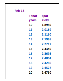
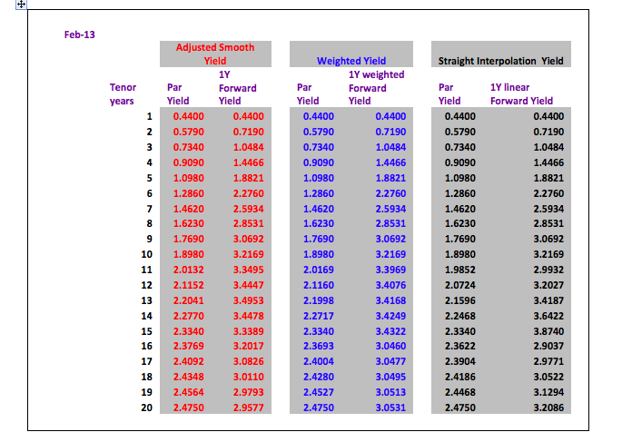
So far in this series we have constructed yield curves based on Interest Rate Swaps. This route was chosen as Swaps provide the benchmark for pricing many loan products. Let us look at constructing a yield curve for local authority loans. Yet again, the choice has been made for a product where prices are published on a daily basis.

The data that is published is not as comprehensive as that for Swaps but, using the procedures shown before, we are still able to build a curve. Only 3 data points were published – 1 year, 5 year and 10 year. It is thus possible to build a 10 year curve – the data is as follows:


Going back to the principles employed when building the IRS curve we shall make a first attempt by using linear interpolation of the spreads – a reasonably obvious approach. I shall save you all the calculations and simply say that this approach leads to an implied 1 year constant maturity curve that is not completely smooth – there is a peak in the period starting in 4 years.

Obviously you could manually alter the prices to achieve a better curve or make use of a curve building model like Nelson & Siegel. Personal experience has resulted in my preference being to calculate the ratio between the local authority rates and the swap rates and allowing the model to find a best fit. Ratios are generally less volatile than the input rates allowing for a better fit. Eventually an implied local authority curve can be built as shown below:

Schermafbeelding 2016-06-20 om 12.37.42

As previously shown the spread is also monotonic – constantly rising. Consider the implications if we know that a 10 year loan has a spread of 70 basis points over swaps whilst the 1 year loan has a spread of only 2 basis points over swaps.

A 10 year spread can also be defined as the weighted average of all the underlying 1 year constant maturities, so let us investigate how this works in this model:

Schermafbeelding 2016-06-20 om 12.37.51

A 10 year spread of 70 basis points starts with a spread of 2 basis points in the 1st year rising in the 10th year to 131 basis points when compared to the underlying implied 1 year constant swap curve. As a treasurer it is important to know how rates are constructed and determine for yourself what the best approach is to your funding needs. Where do you think rates will be in the future, what will the spreads be, borrow for 10 years or borrow for 5 years and renegotiate? A fixed spread is therefore very advantageous for the lender.

No one knows the future but the ability to calculate the implied future price can assist in making decisions now regarding the future. Long dated fixed loans are difficult to break open leading to potential opportunity losses. Bullet loans are the easiest to price, but by focusing only on the cash flows and not their individual time buckets it is possible that the best decisions are not always made. Linear loans are less transparent when pricing but, yet again, a different time approach can be used to make the process simpler. Rollercoaster loans used in construction and infrastructure projects are the most opaque but can also be viewed in a different light if approached in another manner.

Next – Opportunity loss/profit. If I could turn back time or see into the future


Lionel Pavey


Lionel Pavey

Cash Management and Treasury Specialist – Flex Treasurer


Yield Curves (term structure of interest rates) – filling in the blanks part II

| 03-06-2016 | Lionel Pavey |

Most treasurers do not have access to a dedicated financial data vendor (Bloomberg, Reuters) but are regularly faced with having to discover prices related to yield curves. There are websites that can provide us with relevant data, but these are normally a snapshot and not comprehensive – the data series is incomplete. It is therefore up to the treasurer to complete the series by filling in the blanks. In my previous article I went over the first approach. Today I’ll talk about the second approach.

A second approach would be to apply a weighting to the known periods of the par curve and to average the difference out over the missing periods.

grafiek1_part2

Schermafbeelding 2016-06-02 om 13.49.46

This leads to 1 year constant maturity rates that are almost equal in value for all the periods between 2 known periods. Whilst these forward rates are also not correct they at least supply us with a visual indicator as to the general shape of the forward yield curve – the 1 year constant maturity rates

reach their zenith between years 12 and 14; after that point they then start to decrease.

Futhermore, taking into consideration the yield curve as shown in the graph, we can make the following conclusions about the 1 year curve:-

  • 11 year rate must be higher than the linear interpolated rate but lower than the weighted interpolated rate
  • 13 year rate must be higher than the weighted interpolated rate
  • 15 year rate must be lower than the linear interpolated rate and lower than the weighted interpolated rate
  • 16 year rate must be higher than the linear interpolated rate and higher than the weighted interpolated rate
  • 20 year rate must be lower than the linear interpolated rate and lower than the weighted interpolated rate
  • The implied forward 1 year constant maturity curve must be smooth and monotonic.

On the basis of these restraints a par curve can be built that leads to the following forward curve.

grafiek2_part2Schermafbeelding 2016-06-02 om 13.50.01

The rates for the missing periods have been calculated manually whilst adhering to the conditions mentioned before– there are formulae which would allow rates to be discovered (Cubic spline, Nelson Siegel etc.) – but these rely on random variables and I have yet to see anyone quote and trade prices based solely on a mathematical formulae.

Visually, the 1 year curve meets all the criteria for the construction of a yield curve, together with the underlying par and zero yield curves.

grafiek3_part2


To ascertain that the rates are correct, discount all the cash flows of the par yield for the given maturity – they should equal 100.

Here is an overview of all the implied 1 year rates using the different methods to construct the yield curve.

Conclusion:

For a quick calculation a straight line interpolation is acceptable with the warning that with a normal positive yield curve the real prices will be higher than the prices calculated by straight line interpolation. For a negative yield curve this would be reversed – real prices lower than interpolated prices.

The average difference between the par yield prices of the adjusted smooth yield and the straight interpolation yield are only 2.5 basis points. However, this difference is magnified when looking at a 1 year forward yield curve where the average difference is 22.5 basis points per period with a maximum of 53.5 basis points.

Next – Zero Coupon Yields and implied Forward Yields

Would you like to read part one of this article?
– Yield Curves (term structure of interest rates) – filling in the blanks


Lionel Pavey


Lionel Pavey

Treasurer


In de praktijk: Derivaten in de zorgsector

| 30-05-2016 | Willem van Overveld |

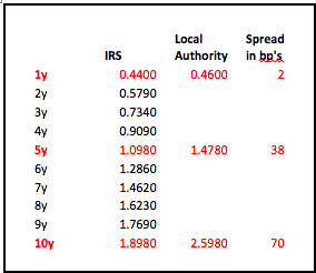
Willem van Overveld beschrijft hoe een simpele SWAP constructie zonder margin calls toch lastig kan worden: de menselijk organisatorische kant van derivaten constructies krijgt vaak te weinig aandacht. Een voorbeeld uit de praktijk:


Het jaar 2012-2013: In een niet nader te noemen financieel zeer rendabel en solvabel ziekenhuis in midden Nederland was een bouwproject gaande ter grootte van 280 mln. euro. Het was vanwege marktomstandigheden niet mogelijk geweest om het financieringsvolume met gangbare leningen aan te trekken. De externe treasury adviseur had aangegeven dit tekort op te kunnen lossen met een renteswap. Onder toeziend oog van toezichthouders werd een renteswap aangekocht, die stapsgewijs opbouwde tot deze 280 mln., en in twintig jaar tijd weer afloste.

De renteswap wisselde 3 maands Euribor voor 3,5% lang met een risico-opslag. Tranches kasgeld onder de renteswap werden aangetrokken met de bouwfacturen die wekelijks binnenstroomden volgens een vaststaand schema. Voordat er een bouwfactuur werd goedgekeurd, werd er een rondleiding op de bouwlocatie gehouden met een bouwkundig opzichter die ook affiniteit had met bancaire diensten. Een extra bankmedewerker was ingehuurd om de verlenging van de kasgelden voor ons uit handen te nemen.

Zo op het eerste gezicht leek de derivatenconstructie een win-win situatie voor alle partijen. Het ziekenhuis kon bouwen en betaalde een vaste nette rente, de bank kon financieren, verdiende op het hoogtepunt 2,8 mln. per jaar (1% winstopslag op een volume van 280 mln.) en de groeiende Vinex wijk was verzekerd van passende zorg. De ratio’s van het ziekenhuis liepen netjes en voorspelbaar binnen alle grenswaarden die met de banken en WSF waren afgesproken.

Voordat ik aantrad als vaste treasury officer was de situatie aan het kantelen. De bedenker van de constructie en de HEAD waren van baan gewisseld en het ziekenhuis had er geen rekening mee gehouden dat er schaarse kennis nodig is om een dergelijke constructie goed te kunnen administreren. De enige persoon die die kennis had was de HEAD zelf, gesteund door externe adviseurs. Zo was men in het ziekenhuis wel op de hoogte dat de IRS (de swap van Rob heette die inmiddels) steeds hogere rentebetalingen vergde, maar men wist niet dat er ook daadwerkelijk geld opgenomen moest worden. (Er is voldoende liquiditeit op de bank en lenen doe je zo min mogelijk toch?) Het gevolg was een SWAP met een verschil tussen werkelijk opgenomen kasgeld van zo’n 60-70 mln. euro.

Een inefficiënte SWAP, waarbij je rente betaalt voor bedrag ‘x’ en kasgeld hebt opgenomen voor bedrag ‘y’ is prettig voor een bank, en hoeft ook nog geen echt probleem te zijn voor een ziekenhuis als de rente niet te hoog of te laag is. Bij mijn aantreden was de Euribor al hard op weg om naar 0 te gaan. Het gevolg was dat de marktwaarde van de SWAP zeer negatief was. We wisselden 3,5% rente voor 0% Euribor: een dure verzekering. Mede ook omdat de effectieve rente over het opgenomen bedrag tussen de 6 en 7 procent lag ontstond er een situatie die aan de toezichthouders niet meer uit te leggen was.

Ik kreeg de instructie om dit probleem op te lossen. Tijdens mijn proeftijd begon ik al de noodzakelijke beleidsrapporten te schrijven, bouwfacturen te verzamelen en liquiditeiten ter grootte van 40 mln. op te nemen. Doel daarvan was om niet in de jaarrekening te hoeven vermelden dat de marktwaarde van de swap 60 mln. negatief was. De accountant kreeg de opdracht een RFP uit te schrijven. Kostprijs hedge accounting kun je alleen toepassen bij een swap die redelijk nominaal loopt. Omdat facturen voorspelbaar waren, was dat gedeelte in een paar weken door mij opgelost. Echter er was ook een vrij te besteden tranche van 23,5 mln. voor vaste medische apparatuur in het nieuwe ziekenhuis maar er was geen investeringsbegroting naar de inkoopafdeling gegaan. Inkopers zijn opgegroeid met Hollandse zuinigheid. Zij moesten tegen hun vakprincipes in zoveel mogelijk geld uitgeven voor medische apparatuur die zij wellicht in goede staat elders in het ziekenhuis konden vinden.

Op het hoogtepunt van mijn interventie stond er 60 mln. aan liquiditeiten op de bankrekening. Om ons heen vielen allerlei bedrijven om door liquiditeitsproblemen. Bij ons liep het geld langs de muren naar beneden. Even hebben we getwijfeld of we zelf geen bank moesten spelen. Dat leverde meer op dan de 0,2% rente die we zelf ontvingen op onze rekening courant. Ik kreeg geen mandaat om gedeelten van het geld elders onder te brengen: te lastig, risicovol, niet conform treasury statuut etc.

Ook in de rentenacalculatie waren er dingen mis gegaan. Ik ontdekte dat er 1,5 mln. euro te weinig was nagecalculeerd aan de broodheren van het ziekenhuis: de zorgverzekeraars. Ook hier had de Hollandse zuinigheid een rol gespeeld: bruto swapbedragen betalen en netto bedragen nacalculeren. NZA (Nederlandse Zorg Autoriteit) oordeelde dat er een lek in de wetgeving was ontstaan en ze geen middelen hadden om een ziekenhuis te ontzeggen de bruto SWAP bedragen in rekening te brengen. Wij zetten door en kregen ons gelijk. We hadden snel 1,5 mln. verdiend. Na deze reparatie actie werd mij een andere baan aangeboden.

Ik hoorde dat de NZA was ingevallen in de week nadat ik van baan was gewisseld. Dit had niets met treasury te maken, maar met verkeerd gedeclareerde zorgproducten. Het ziekenhuis kreeg 20 mln. euro boete opgelegd. Gelukkig had het betreffende ziekenhuis genoeg liquiditeit op de bank staan op dat moment.

De veelbelovende, maar wat stagnerende Vinex wijk waarin gebouwd werd, is later qua bouwvolume woningen ook bijgetrokken.

Willem van Overveld – Allround finance / treasury professional
[social_links size=”normal” align=””  linkedin=”https://www.linkedin.com/in/willemvanoverveld”]