Workshop: Treasury Systems – het waarom en hoe (niet) van Treasury & Banking Software
| 02-06-2016 | treasuryXL
 Op 26-05-2016 waren treasuryXL en Treasurer Search aanwezig op Financial Systems. Naast dat we een stand op de beursvloer hadden, hebben we ook een invitation only sessie georganiseerd: Treasury Systems – het waarom en hoe (niet) van Treasury & Banking Software. Hiervoor hebben we vier interim managers uitgenodigd die elk hun eigen gekozen topics kwamen pitchen. De deelnemers van de workshop waren vrij om vragen te stellen en aan te vullen waar nodig. Het resultaat was een geslaagde en interactieve sessie waaruit we ook voor treasuryXL inspiratie konden putten.
Op voorhand hebben we een aantal doelen gesteld voor deze sessie:
- Ontwikkelingen op het snijvlak Treasury & Financial Systems doornemen
- Voor leken: overview & duiding
- Voor experts: verdere verdieping en bruggen slaan
- Voor treasuryXL: inventarisatie informatiebehoefte
- Voor allen: bepalen met wie je mogelijk volgende stappen wilt zetten
De vier interim managers aan het woord
Hieronder volgt een korte samenvatting van de presentaties van de vier interim managers met (indien aanwezig) reacties uit de zaal.
Erik Teiken
 Accounting in je TMS – zijn er voordelen?
Een TMS heeft vaak accounting modules maar deze worden niet altijd vanaf het begin meegenomen voornamelijk vanwege de kosten en extra tijd en inspanning voor de inrichting ervan. Toch zijn er wel voordelen voor het meenemen van een accounting module in je TMS en na verloop van tijd wordt er vaak toch tot aanschaf overgegaan. Dit heeft volgens Erik te maken met drie punten:
- Na intensiever gebruik blijkt de accounting module toch nodig door de hoeveelheid deals, wat lastig aan te sluiten is met ERP.
- Ook de complexiteit van bijvoorbeeld exotische deals heeft vaak invloed. Door een accounting module kun je alle verplichtingen in je TMS ook meenemen.
- Ook Hedge Accounting volgens IFRS heeft zo zijn voordelen bij het implementeren van een accounting module, het wordt makkelijker te automatiseren. De treasurer wil inzicht in eigen p&l verantwoording, EMIR.
Marktsystemen – toeters en bellen?
Er zitten natuurlijk voordelen aan het aanschaffen van een systeem als Reuters of Bloomberg. Het levert de treasurer actuele marktinformatie op; informatie over valuta´s, interest en nieuws. Op langere termijn kun je zien hoe de yield curve loopt en levert het toegevoegde waarde op; je kunt scenario’s ontwikkelen over exposure in de toekomst en daar kun je je strategie op aanpassen. Er zijn toeters en bellen die waarschuwen. Een nadeel van het aanschaffen van een marktsysteem is het kostenplaatje: zo’n 15-20K per jaar.
Static Data in je TMS – levert het wat op?
Static data lijkt het ondergeschoven kindje te zijn in een TMS, en wordt als droog en saai ervaren. Het gevaar van je static data niet op orde hebben is dat je veel tijd verliest met zoeken van essentiële data. Geen match met ERP is nog wel te overkomen maar wat als betalingen op verkeerde rekeningen terecht komen of niet uitgevoerd kunnen worden?
Het is dus van belang dit op orde te hebben maar ook om functiescheiding toe te passen; iemand voert in en iemand controleert de invoer. In treasury kan elke fout kostbaar zijn voor een bedrijf.
Menno van Suylichem
 Welke variabelen bepalen je systeemkeuze?
De doelen van een implementatie zijn kostenreductie, efficiency en risicobeperking. Variabelen die de systeemkeuze bepalen zijn onder meer: cloud versus stand-alone applicatie, functionaliteiten, modulaire opbouw, integratie met bestaande ERP systemen, reporting tools, ondersteuning leverancier, toegankelijkheid en kosten.
Voordat je überhaupt kan overgaan tot implementatie dienen de bestaande static (basis) data goed bereikbaar te zijn en gecontroleerd te worden, eventueel aangevuld met nieuwe informatie. Houdt hierbij zoveel mogelijk rekening met nieuwe (toekomstige) functionaliteiten/gebruik van het systeem.
Wat wil ik als bedrijf, wat heb ik echt nodig aan informatie, nu en in de nabije toekomst. Niet alle applicaties van een systeem zijn (direct) van toepassing. Start met de meest noodzakelijke, d.w.z. de applicaties die de dagelijkse processen en de daaruit voortvloeiende beslissingen/risico’s direct ondersteunen en beperken.
Implementatie outsourcen of zelfstandig?
Bedrijven onderschatten vaak hoeveel tijd het kost om een TMS zelf te implementeren. Reken op 12 tot 18 maanden, waarbij een persoon binnen de organisatie moet worden vrijgemaakt. Deze kennis verdwijnt vervolgens als diegene van functie veranderd of het bedrijf verlaat
Uit de zaal komt de input dat je bij het zelf implementeren alles zelf in de hand hebt, bij outsourcing zit de leverancier er niet zo midden in en weet dus niet exact wat er wel en niet nodig is. Reactie hierop is dat een goede blueprint van belang is en dat je de leverancier duidelijk opdracht kan geven over wat jij wel of niet wilt.
Inrichting systeem moet binnen de bestaande procuratieschema’s passen
Het is belangrijk de toegang tot een TMS goed in te richten. Houd ook in de gaten hoe het voorheen zat; wie mag transacties invoeren, wie mag transacties afsluiten, wie mag deze transacties invoeren en wie mag de hieruit voortvloeiende betalingsopdrachten tekenen? Meerdere mensen geven aan vaker tegen procuratie aan te lopen. Vooral omdat ze in de praktijk nog nooit hebben meegemaakt dat het hiermee mis ging.
Procedurele controle is belangrijk, dit wordt ook door de deelnemers in de zaal bevestigd, altijd alles met gescheiden autorisatie; één persoon voert in en één persoon geeft akkoord.
Dick Bennink
 Systeem dwingt altijd tot aanpassingen in huidige proces – wees voorzichtig met customizen
Doe aan pakketselectie. De leverancier zegt misschien dat het kan maar tijdens de daadwerkelijke implementatie blijkt toch dat het net niet kan of helemaal niet kan. De mensen die werken bij de leveranciers zijn niet altijd werkzaam in treasury, en sluiten niet altijd goed aan op de praktijk. Systemen zijn niet perfect, probeer een balans te vinden in het veranderen of de kleine aanpassing. Blijf uit de buurt van hele grote veranderingen. Dit brengt hoge kosten met zich mee en maatwerk leidt tot een hoop extra werk.
“Meenemen” en “meekrijgen” van alle (internationale) ondernemingen bij een implementatie
Implementeren blijkt vaak een ‘hoofdkantoor-feestje’ te zijn, je bent afhankelijk van dochterondernemingen. Hoofdzaak is om mensen lager in de organisatie te laten helpen om de implementatie tot een succes te maken. Luister naar de dochterondernemingen om te zorgen dat de workload die jij aan ze oplegt om het systeem te voeden, te doen is. Kijk of er dingen in het systeem zijn die je terug kunt geven, bijvoorbeeld om de werkzaamheden makkelijker of efficiënter te laten verlopen. Zorg voor een duidelijke blueprint om aanpassingen in het lopende proces te minimaliseren. Onafhankelijk van wat je doet, zorg dat je binnen 3 maanden succes kunt vieren.
Olivier Werlingshoff
 Systemen maar Cash Awareness is de basis!
Cash awareness is belangrijk, er wordt veel gehamerd op TMS, rapportages en analyses. De basis is dat datgene dat ingevoerd wordt voor de liquiditeitsplanning ook zorgt voor een goede planning.
Bij liquiditeitsplanningen is de business leidend en niet de systemen
Collega’s uit de organisatie weten vaak veel beter wanneer bepaalde stromen werkelijk binnen zullen komen en eruit zullen gaan. Hetgeen dat de business aangeeft is bepalend voor de planning.
Toegang tot de TMS voor de Business
Het kan handig zijn om bij input vanuit de business de persoon verantwoordelijk te maken voor hetgeen waar ze input voor hebben gegeven, zo creëer je cash awareness binnen de organisatie omdat mensen zich betrokken voelen, verantwoordelijkheid voelen voor hetgeen ze hebben aangegeven en veranderingen worden sneller doorgegeven. Tot slot is het hiervoor handig om toegang tot de TMS te geven aan collega’s uit de business om de input te kunnen doorgeven en/of de planning te kunnen controleren.
De sessie samengevat
Het was een geslaagde, interactieve workshop die nieuwe inzichten met zich meebracht. Samen met de aanwezigen waren we het er over eens dat er een aantal onderwerpen zijn waarbij nog meer verdieping nodig is:
- Static data
- Integratie tussen systemen
- Blueprint
- Procuratie
- Cash awareness, (vergeten kindje, koppelen met business)
- Surrealistische gesprekken met leveranciers.
- Binnenhengelen onderliggende partij, geven en nemen
Over deze onderwerpen zullen in de komende tijd dan ook artikelen verschijnen op treasuryXL. Heb je interesse om een artikel te schrijven over een van deze onderwerpen? Neem dan contact met mij op via [email protected].
Ook namens Treasurer Search willen we alle aanwezigen bedanken voor hun komst en input. We hopen in de toekomst meer van deze interessante sessies te kunnen organiseren.
 Stephanie Derkse
Community Manager
[email protected]
06-21303744
 On april 13th of this year the Fintech innovation awards took place. Vallstein won the innovation award in treasury management with their Walletsizing® system. We asked Huub Wevers from Vallstein to give us an update on this new system. What’s new about it and who will benefit from using Walletsizing®?
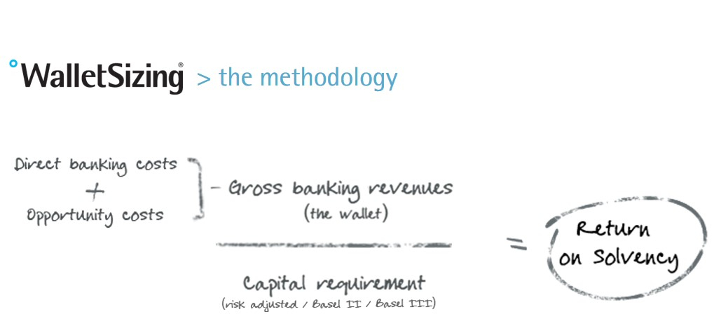
 Huub Wevers is responsible for Corporate Solutions at Vallstein, the leading Bank Relationship Management specialist. Before joining Vallstein he has had eighteen years of experience in Banking at ABN AMRO and RBS, notably Transaction Banking. His responsibilities included Product Management, Account Management, Implementation and Operations, whereby his last role was the leadership of all Service & Operations in EMEA for RBS. At Vallstein Huub is responsible for building out the software solutions that Vallstein offers for corporates. Solutions that automate bank relationship management in order to assess the profitability that a corporate has for their banks, using all banking products and Basel III.
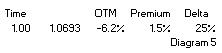 (1.5%, see diagram 5) by the chance it will be exercised (Delta, in this case 25%), ie 1.5% : 25% = 6%. It could be a very disappointing to find that if this Conditional Premium option is only marginally ITM at maturity, because the premium of 6% still has to be paid.
 Willem van Overveld beschrijft hoe een simpele SWAP constructie zonder margin calls toch lastig kan worden: de menselijk organisatorische kant van derivaten constructies krijgt vaak te weinig aandacht. Een voorbeeld uit de praktijk:
 Willem van Overveld – Allround finance / treasury professional


 Last week I visited an information session about financial postgraduate education. It was organized by the VU (Vrije Universiteit, Amsterdam). I noticed an increased interest in comparison to last years session, which is great. Information was provided about courses I see back in the CV’s of treasurers: CFA, RBA (Register Belegging Analyst) and of course RT (Register Treasurer) that has an overlap with the ACT courses. Education, specifically postgraduate, is a topic that returns in many of my meetings. This is what I notice on the topic:
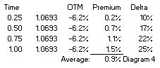
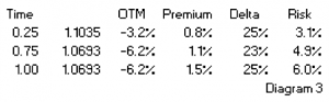 bought the option for 1.5%, we could sell it after 3 months at 1.1% and buy the USD through an outright forward transaction. This approach shows that the net cost of option protection would be only 0.4% (1.5% – 1.1%). Which would be cheaper than the premium of a 3-month option with the same Delta. Also, because the option has a higher Delta than a 3-month option with the same strike (25% vs 10%, see diagram 2), it will follow the spot market much better. The bottom line of paragraph 3 is that a longer dated option can be bought with the intention to sell it again at some point, the net cost being less than buying a shorter dated option. While it serves as a hedge against price changes.
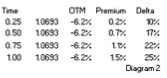 buy the 1-year option in diagram 2 for 1.5%. Alternatively we could consider buying a right to buy this option for 0.4% in 3 months time. At that time the 1-year option will only have 9 months remaining, but the strike and 1.5% premium are fixed in the contract. On the expiry date of the compound option we can decide if we want to pay 1.5% for the underlying option. Alternatively, assuming nothing has changed, we could buy a 9 month option in the market for 1.1% (see diagram 2). In such a case we wouldn’t exercise the compound option.