Yield Curves (term structure of interest rates) – filling in the blanks part II
| 03-06-2016 | Lionel Pavey |
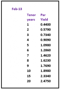
Most treasurers do not have access to a dedicated financial data vendor (Bloomberg, Reuters) but are regularly faced with having to discover prices related to yield curves. There are websites that can provide us with relevant data, but these are normally a snapshot and not comprehensive – the data series is incomplete. It is therefore up to the treasurer to complete the series by filling in the blanks. In my previous article I went over the first approach. Today I’ll talk about the second approach.
A second approach would be to apply a weighting to the known periods of the par curve and to average the difference out over the missing periods.
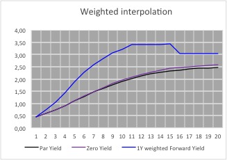
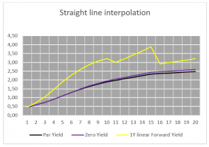
This leads to 1 year constant maturity rates that are almost equal in value for all the periods between 2 known periods. Whilst these forward rates are also not correct they at least supply us with a visual indicator as to the general shape of the forward yield curve – the 1 year constant maturity rates
reach their zenith between years 12 and 14; after that point they then start to decrease.
Futhermore, taking into consideration the yield curve as shown in the graph, we can make the following conclusions about the 1 year curve:-
- 11 year rate must be higher than the linear interpolated rate but lower than the weighted interpolated rate
- 13 year rate must be higher than the weighted interpolated rate
- 15 year rate must be lower than the linear interpolated rate and lower than the weighted interpolated rate
- 16 year rate must be higher than the linear interpolated rate and higher than the weighted interpolated rate
- 20 year rate must be lower than the linear interpolated rate and lower than the weighted interpolated rate
- The implied forward 1 year constant maturity curve must be smooth and monotonic.
On the basis of these restraints a par curve can be built that leads to the following forward curve.
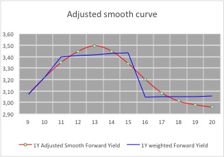
The rates for the missing periods have been calculated manually whilst adhering to the conditions mentioned before– there are formulae which would allow rates to be discovered (Cubic spline, Nelson Siegel etc.) – but these rely on random variables and I have yet to see anyone quote and trade prices based solely on a mathematical formulae.
Visually, the 1 year curve meets all the criteria for the construction of a yield curve, together with the underlying par and zero yield curves.
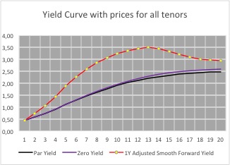
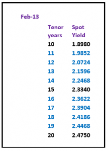
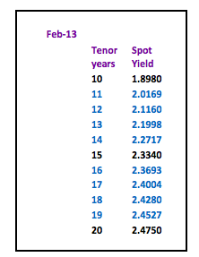
To ascertain that the rates are correct, discount all the cash flows of the par yield for the given maturity – they should equal 100.
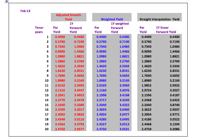
Here is an overview of all the implied 1 year rates using the different methods to construct the yield curve.
Conclusion:
For a quick calculation a straight line interpolation is acceptable with the warning that with a normal positive yield curve the real prices will be higher than the prices calculated by straight line interpolation. For a negative yield curve this would be reversed – real prices lower than interpolated prices.
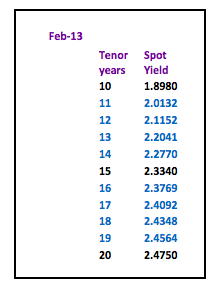
The average difference between the par yield prices of the adjusted smooth yield and the straight interpolation yield are only 2.5 basis points. However, this difference is magnified when looking at a 1 year forward yield curve where the average difference is 22.5 basis points per period with a maximum of 53.5 basis points.
Next – Zero Coupon Yields and implied Forward Yields
Would you like to read part one of this article?
– Yield Curves (term structure of interest rates) – filling in the blanks

Treasurer