Tag Archive for: interest rate

How are largest European companies managing their financial risks?

17-10-2019 | Stanley Myint | BNP Paribas

The second edition of the “Handbook of Corporate Financial Risk Management” has just been published by Risk books. The handbook is written with all risk management professionals, practitioners, instructors and students in mind, but its core readership are Treasurers at non-financial corporations. It contains 43 real life case studies covering various risk management areas. The book aims to cover both financial risk management and optimal capital structure and its contents.

Motivation for the book

This Handbook is based on real-life client discussions we had in the Risk Management Advisory team at BNP Paribas between 2005 and 2019. We noticed that corporate treasurers and chief financial officers (CFOs) often have similar questions on risk management and capital structure and that these questions are rarely addressed in the existing literature.

This situation can and should lead to a fruitful collaboration between companies and their banks. Companies often come with the best ideas, but do not have the resources to test them. Leading banks, on the other hand, have strong computational resources, a broader sector perspective, an extensive experience in internal risk management, and the ability to develop and deliver the solution. So, if they make an effort to understand a client’s problem in depth, they may be able to add considerable value.

The Handbook is the result of such an effort lasting 14 years and covering more than 700 largest European corporations from all industrial sectors. Its subject is corporate financial risk management, ie, the management of financial risks for non-financial corporations.

While there are many papers on this topic, they are generally written by academics and rarely by practitioners. If we contrast this to the subject of risk management for banks, on which many books have been written from the practitioners’ perspective, we notice a significant gap. Perhaps this is because financial risk is clearly a more central part of business among banks and asset managers than in non-financial corporations. However, that does not mean that financial risk is only important for banks and asset managers. Let us look at one example.

Consider a large European automotive company, with an operating margin of 10%. More than half of its sales are outside Europe, while its production is in EUR. This exposes the company to currency risk. Annual currency volatility is of the order of 15%, therefore, if the foreign revenues fall by 15% due to FX, this can almost wipe out the net profits. Clearly an important question for this company is, “How to manage the currency risk?”

The book blends real corporate situations across capital structure, optimal level of cash, optimal fixed-floating mix and pensions, which are particularly topical now that negative EUR yields create unpresented funding opportunities for corporates, but also tricky challenges on cost of cash and pensions management

One reason why corporate risk management has so far attracted relatively little attention in literature is that, even though the questions asked are often simple (eg, “Should I hedge the translation risk?” or “Does hedging transaction risk reduce the translation risk?”) the answers are rarely simple, and in many cases there is no generally accepted methodology on how to deal with these issues.

So where does the company treasurer go to find answers to these kinds of questions? General corporate finance books are usually very shy when it comes to discussing risk management. Two famous examples of such books devote only 20 – 30 pages to managing financial risk, out of almost 1,000 pages in total. Business schools generally do not devote much time to risk management. We hope that our book goes a long way towards filling this gap.

Website

We invite the reader to utilise the free companion website which accompanies this book, www.corporateriskmanagement.org There, you will find periodic updates on new topics not covered in The Handbook. Much like the book this website should prove a useful resource to corporate treasurers, CFOs and other practitioners as well the academic readers interested in corporate risk management.

About the authors

Stanley Myint is the Head of Risk Management Advisory at BNP Paribas and an Associate Fellow at Saïd Business School, University of Oxford. At BNP Paribas, he advises large multinational corporations on issues related to risk management and capital structure. His expertise is in quantitative and corporate finance, focusing on fixed income derivatives and optimal capital structure. Stanley has 25 years of experience in this field, including 14 years at BNP Paribas and previously at McKinsey & Company, Royal Bank of Scotland and Canadian Imperial Bank of Commerce. He has a PhD in physics from Boston University, a BSc in physics from Belgrade University and speaks French, Spanish, Serbo-Croatian and Italian. At the Saïd Business School, Stanley teaches two courses with Dimitrios Tsomocos and Manos Venardos: “Financial Crises and Risk Management” and “Fixed Income and Derivatives”.

Fabrice Famery is Head of Global Markets corporate sales at BNP Paribas. His group provides corporate clients with hedging solutions across interest rate, foreign exchange, commodity and equity asset classes. Corporate risk management has been the focus of Fabrice’s professional path for the past 30 years. He spent the first seven years of his career in the treasury department of the energy company, ELF, before joining Paribas (now BNP Paribas) in 1996, where he occupied various positions including FX derivative marketer, Head of FX Advisory Group and Head of the Fixed Income Corporate Solutions Group. Fabrice has published articles in Finance Director Europe and Risk Magazine, and has a master’s degree in international affairs from Paris Dauphine University (France).

Content:

Introduction

1 Theory and Practice of Corporate Risk Management *

2 Theory and Practice of Optimal Capital Structure *

PART I: FUNDING AND CAPITAL STRUCTURE

3 Introduction to Funding and Capital Structure

4 How to Obtain a Credit Rating

5 Refinancing Risk and Optimal Debt Maturity*

6 Optimal Cash Position *

7 Optimal Leverage *

PART II: INTEREST RATE AND INFLATION RISKS

8 Introduction to Interest Rate and Inflation Risks

9 How to Develop an Interest Rate Risk Management Policy

10 How to Improve Your Fixed-Floating Mix and Duration

11 Interest Rates: The Most Efficient Hedging Product*

12 Do You Need Inflation-linked Debt

13 Prehedging Interest Rate Risk

14 Pension Fund Asset and Liability Management

PART III: CURRENCY RISK

15 Introduction to Currency Risk

16 How to Develop an FX Risk Management Policy

17 Translation or Transaction: Netting FX Risks *

18 Early Warning Signals

19 How to Hedge High Carry Currencies*

20 Currency Risk on Covenants

21 Optimal Currency Composition of Debt 1:

Protect Book Value

22 Optimal Currency Composition of Debt 2:

Protect Leverage*

23 Cyclicality of Currencies and Use of Options to Manage Credit Utilisation *

24 Managing the Depegging Risk *

25 Currency Risk in Luxury Goods *

PART IV: CREDIT RISK

26 Introduction to Credit Risk

27 Counterparty Risk Methodology

28 Counterparty Risk Protection

29 Optimal Deposit Composition

30 Prehedging Credit Risk

31 xVA Optimisation *

PART V: M&A-RELATED RISKS

32 Introduction to M&A-related Risks

33 Risk Management for M&A

34 Deal-contingent Hedging *

PART VI: COMMODITY RISK

35 Introduction to Commodity Risk

36 Managing Commodity-linked Revenues and Currency Risk

37 Managing Commodity-linked Costs and Currency Risk

38 Commodity Input and Resulting Currency Risk *

39 Offsetting Carbon Emissions*

PART VII: EQUITY RISK

40 Introduction to Equity Risk*

41 Hedging Dilution Risk *

42 Hedging Deferred Compensation*

43 Stake-building*

Bibliography

Index

Note: Chapters marked with * are new to the second edition

Best read articles of all time – Beleggen in obligaties met een hoge rente – een bespiegeling

|09-05-2018 | Douwe Dijkstra – Fastned- Het Financieele Dagblad |

pile-of-money


Hoe interessant is beleggen in bedrijfsobligaties met een hoge rente? Hoe aantrekkelijk is deze financieringsoptie voor ondernemingen? Wij  hebben onze experts Douwe Dijkstra en Pieter de Kiewit om een kort commentaar gevraagd naar aanleiding van de obligatie uitgifte van Fastned.


Op de site van Fastned was begin december 2016 te lezen:
‘U kunt nu investeren in Obligaties Fastned met 6% rente’. Later in de maand ging de tekst verder: ‘We zijn verheugd u te kunnen mededelen dat Fastned de inschrijving is gestart voor de uitgifte van obligaties. De obligaties hebben een looptijd van 5 jaar en keren per jaar 6% rente uit. Dit is een mooie kans om (verder) te investeren in de groei van Fastned en een duurzame wereld.’
Vervolgens werden de belangrijkste kenmerken van Obligaties Fastned genoemd.
Dat de obligaties zeer gewild waren blijkt vandaag. Op de site van Fastned verschijnt nu een tekst dat alle obligaties geplaatst zijn. En Fastned vervolgt:
‘Gezien de grote interesse in obligaties Fastned zijn er zeker voornemens om binnenkort nog een uitgifte te doen.’

In het Financieele Dagblad kon men op 6 december een Bartjens commentaar lezen over de Fastned obligaties:  Het principe is simpel: een wankel bedrijf leent geld. Beleggers willen de relatief grote kans op wanbetaling gecompenseerd zien met een behoorlijke vergoeding: dus een hoge rente. In de VS zijn junkbonds populair, hier is het een kleine markt. Maar deze week is er weer een onvervalst speculatieve obligatie uitgegeven. Fastned. Het bedrijf dat een Europees netwerk van snellaadstations voor elektrische auto’s bouwt, leende € 2,5 mln. De lening heeft een looptijd van vijf jaar. De couponrente is 6%. Ter vergelijking: de Nederlandse Staat (superveilig) leent voor vijf jaar tegen 0%, Shell (behoorlijk veilig) leent voor vijf jaar tegen een coupon van 1,25% en Gazprom (Russisch, iets minder veilig) leent in Zwitserse frank voor vijf jaar tegen 2,75%. De 6% van Fastned impliceert dus behoorlijke risico’s. Het bedrijf is klein, jong en verlieslatend. Het heeft geen reserves en een negatief eigen vermogen, zo blijkt uit het prospectus. Maar goed, ‘de cost gaet voor de baet uyt’ en juist nu moet Fastned investeren.’

Expert Douwe Dijkstra vult hierop aan:
Voor beleggen in Fastned obligaties geldt hetzelfde als voor elke andere investering. Het rendement is omgekeerd evenredig aan het risico. Zolang niemand weet of de koers van aandelen Koninklijke Olie omhoog of naar beneden gaan, weet zeker niemand of beleggen in een 6% obligatie van Fastned achteraf wel of geen goede investering zal blijken te zijn geweest. Het lijkt mij enkel aantrekkelijk voor beleggers die wel een gokje durven te wagen met een te overziene inzet die ze wel kunnen missen. Of voor beleggers met een ideologische wereldvisie. Vorige week las ik in een ander artikel nog dat die investeerders met een loep gezocht moeten worden.

En Pieter de Kiewit zegt:
Investeren in start-ups gaat mijns inziens gepaard met een andere investeringsanalyse dan in volwassen ondernemingen. Daarbij is de ‘groene factor’ voor vele beleggers reden anders naar een onderneming te kijken. Dit is bijvoorbeeld heel zichtbaar bij Tesla. Persoonlijk vraag ik me af of een avontuurlijke investeerder in dit geval niet beter een equity investering kan doen.
Vanuit Fastned perspectief kan ik, met hun vertrouwen in hun business case, begrijpen dat ze liever obligaties uitgeven dan nieuwe aandelen..

douwedijkstra


Douwe Dijkstra

Owner of Albatros Beheer & Management


Forward Rate Agreement (FRA)

| 05-01-2018| Arnoud Doornbos |

Money Market outlook

At the press conference on 14 December 2017, the ECB announced that expectations for economic growth and inflation have been adjusted upwards. But despite optimistic growth, the ECB is not yet fully convinced of a continued upward trend in domestic price pressures. And thus Draghi: “An ample degree of monetary stimulus … is necessary for underlying inflation pressures to continue to build up.”

For this reason, the ECB will maintain the buying program at least until September 2018. And only then will an increase in policy rates come into the picture. Since the beginning of 2017, investors have seen the chance that the ECB will implement an increase in policy interest rates. This has not yet had an effect on the three-month Euribor rate. This has been stable at around -0.3% for the whole of 2017, and we expect that this will be the case in the vast majority of 2018 as well.

But markets will go up again for sure during time and borrowers need to prepare themselves for that moment. A good interest rate risk management can help to extent the pleasure of using favorable low interest rates for your company. Hedging your short term interest rate exposure with FRA’s could be a good idea. Good timing is essential.


Definition

A Forward Rate Agreement’s (FRA’s) effective description is a cash for difference derivative contract, between two parties, benchmarked against an interest rate index. That index is commonly an interbank offered rate (-IBOR) of specific tenor in different currencies, for example LIBOR in USD, GBP, EURIBOR in EUR or STIBOR in SEK. A FRA between two counterparties requires a fixed rate, notional amount, chosen interest rate index tenor and date to be completely specified.

FRAs are not loans, and do not constitute agreements to loan any amount of money on an unsecured basis to another party at any pre-agreed rate. Their nature as a IRD product creates only the effect of leverage and the ability to speculate, or hedge, interest rate risk exposure.


How it works

Many banks and large corporations will use FRAs to hedge future interest or exchange rate exposure. The buyer hedges against the risk of rising interest rates, while the seller hedges against the risk of falling interest rates. Other parties that use Forward Rate Agreements are speculators purely looking to make bets on future directional changes in interest rates.

In other words, a forward rate agreement (FRA) is a tailor-made, over-the-counter financial futures contract on short-term deposits. A FRA transaction is a contract between two parties to exchange payments on a deposit, called the Notional amount, to be determined on the basis of a short-term interest rate, referred to as the Reference rate, over a predetermined time period at a future date.

At maturity, no funds exchange hands; rather, the difference between the contracted interest rate and the market rate is exchanged. The buyer of the contract is paid if the published reference rate is above the fixed, contracted rate, and the buyer pays to the seller if the published reference rate is below the fixed, contracted rate. A company that seeks to hedge against a possible increase in interest rates would purchase FRAs, whereas a company that seeks an interest hedge against a possible decline of the rates would sell FRAs.


Valuation and Pricing

 The cash for difference value on a FRA, exchanged between the two parties, calculated from the perspective of having sold a FRA (which imitates receiving the fixed rate) is calculated as:

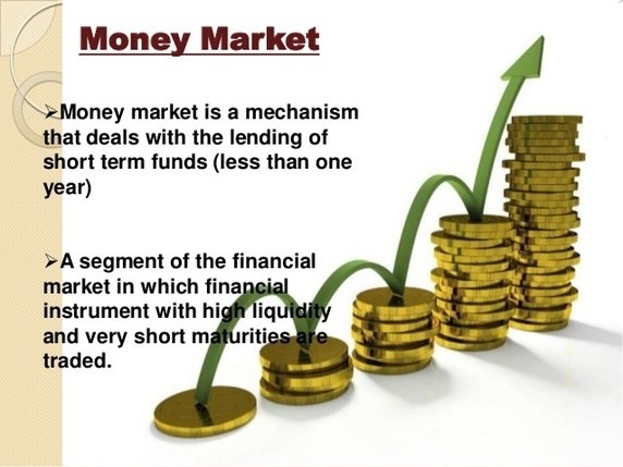
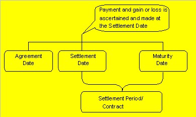
where N is the notional of the contract, R is the fixed rate, r is the published -IBOR fixing rate and d is the decimalized day count fraction over which the value start and end dates of the -IBOR rate extend.

For USD and EUR this follows an ACT/360 convention and GBP follows an ACT/365 convention. The cash amount is paid on the value start date applicable to the interest rate index (depending in which currency the FRA is traded, this is either immediately after or within two business days of the published -IBOR fixing rate).

For mark-to-market (MTM) purposes the net present value (PV) of an FRA can be determined by discounting the expected cash difference, for a forecast value r:

where vn is the discount factor of the payment date upon which the cash for difference is physically settled, which, in modern pricing theory, will be dependent upon which discount curve to apply based on the credit support annex (CSA) of the derivative contract.

Quotation and Market-Making

 FRA Descriptive Notation and Interpretation


How to interpret a quote for FRA?

[EUR 3×6  -0.321 / -0.301%p.a ] – means deposit interest starting 3 months from now for 3 month is -0.321% and borrowing interest rate starting 3 months from now for 3 month is -0.301%. Entering a “payer FRA” means paying the fixed rate (-0.321% p.a.) and receiving a floating 3-month rate, while entering a “receiver FRA” means paying the same floating rate and receiving a fixed rate (-0.321% p.a.).

Due to the current negative Money Market rates means receiving actually paying and the other way around.


Arnoud Doornbos 

Interim Treasury & Finance


Will the ECB taper off its Quantitative Easing programme?

| 23-10-2017 | Lionel Pavey |

On the 26th October the ECB will have their next meeting. One of the main topics will be regarding the current QE programme and a possible announcement over its extension into 2018. Currently the ECB has, after 2 ½ years of QE, purchased more than EUR 2 trillion of mainly Government bonds. At present their monthly purchases amount to roughly EUR 60 billion per month.

A poll organized by Reuters would seem to indicate that the monthly programme would be tapered down to EUR 30-50 billion per month and possibly last for another 6 to 12 months from the start of 2018. Inflation is expected to be around 1.5 per cent till at least the start of 2019 – below the ECB target of just below 2 per cent.

However, under the current rules that govern the QE progamme the upper limit on outstanding purchases is around EUR 2.5 trillion. Taking the existing monthly purchases through to the end of 2017, implies starting 2018 with a balance of at least EUR 2.2 trillion – leaving just EUR 300 billion of headroom for future purchases. If it cut monthly purchases in half, the scheme could be extend to the end of the 3rd quarter in 2018, but no further.

Can the ECB continue QE longer than expected?

The constraints imposed on QE mainly relate to the purchase of Government bonds – maximum 33 per cent of each countries outstanding debt and maximum 25 per cent of any bond issue. The provisions written into the Maastricht Treaty clearly state that the ECB may not finance member states. QE also purchases non-bank bonds (covered bonds, corporate bonds and asset backed securities) which are subject to different criteria – maximum of 70 per cent of any bond issue.
At present, the ECB only holds about 13 per cent of the eligible bonds leaving a large headroom for future possible purchases.

It is conceivable that the ECB could reduce its purchase of Government bonds and simultaneously increase its purchase of corporate bonds, thereby maintaining liquidity to its QE programme. The major drawback is that it would reduce the amount of freely tradable corporate bonds in circulation and have an effect on their price.

What does this mean for interest rates?

As long term debt instruments use Government bond yields as the basis for calculating their yield, when the ECB stops buying Government bonds, the yields on all other debt instruments will increase. At the moment the benchmark (German 10 year Government bonds) yield around 0.4 per cent per annum and the 10 year Interest Rate Swap yields around 0.9 per cent per annum. In 2014 (the year before QE started) German yields averaged 1.25 per cent even though they were in a downward trend the whole year. Assuming the yield spread between Government bonds and Interest Rate Swaps (IRS) remained constant, this implies 10 year IRS moving to at least 1.75 per cent. This would still be below the long term average since the inception of the EURO in 1999 that stands around 3.35 per cent, but a significant increase from the current level of 0.9 per cent.

What happens when the next crisis arrives?

The ECB is not the only central bank to use a form of QE. The Fed, Bank of England and Bank of Japan all have their own versions. When these countries also taper out their QE, naturally there will be a corresponding rise in interest rates. However, if a new financial crisis was suddenly to happen (not unthinkable at the moment) all 3 of these central banks can reapply QE to stimulate their economies. An additional increase to their balance sheets can be accommodated.

Unfortunately for the ECB the very criteria that now applies would make it impossible to restart QE. The ECB could not just increase its balance sheet – current criteria and regulation make that impossible. Any attempt to change the rules would be met by objections from national governments within the EU and legal action. The Bundesbank were very vocal in their objections to the implementation of QE in 2015 – those protests will not have softened by now.

This shows the constraints prevalent upon the EURO – monetary policy is the only tool that the ECB has at its disposal. One policy can not be used to fix all the problems present with the economies of all member states.


Lionel Pavey

Cash Management and Treasury Specialist


Risk Management – what does it mean

| 24-5-2017 | Patrick Kunz |

You might visit this site, being a treasury professional with years of experience in the field. However you could also be a student or a businessman wanting to know more details on the subject, or a reader in general, eager to learn something new. The ‘Treasury for non-treasurers’ series is for readers who want to understand what treasury is all about.
Our expert Patrick Kunz tells us more about an important task of a treasurer: Risk Management

Background

One of the main task of a treasury is risk management, more specifically financial risk management. This is still broad as financial risk can result from many origins. Treasury is often involved in the risk management of Foreign currency (FX), interest rates, commodity prices and sometimes also balance sheet/profit loss. Furthermore insurances are often also the task of the treasurer.

Exposure

To be able to know how to reduce a certain risk the treasurer first needs to know about the risk. Often risk positions are taken outside of the treasury department. The treasurer needs to be informed about these risk positions. FX and commodity price exposure is often created in sales or procurement while the interest rate risk is created in the treasury department itself (although this is not always the case). In an ideal world the treasurer would like to know an exposure right after it is created. Often IT solutions or ERP connections with treasury help with that.

Policy

Once the exposure is know the treasurer needs to decide whether it is a risk position or not and whether he wants to mitigate this risk by hedging it. Let me explain this with an FX example: A EUR company who buys goods in USD is at risk for movements in the EUR/USD rate. However, if the company is able to sell these goods at the same time they are bought (a sales organization), for  USD then the net exposure could be lower. Risk Exposure is therefore lower as only the profit needs to be hedged.

Risk appetite of the company determines if the treasurer needs to take action on certain risk exposure. Some companies hedge all their FX exposure. The reason for this is often because FX risk is not their core business and therefore not a business risk. Non-core risk needs to be eliminated. Commodity risk is sometimes not hedged as this is the company’s core business or a natural hedge as the companies is also producer/miner and seller of the commodity. Other companies have more risk appetite and hedge only amounts above a certain threshold. Due to internal information restrictions, delays or accounting issues and the fact that some currencies are not hedgable most multinationals always have some FX exposure. In the profit and loss statements you often see profit or losses from FX effect, either realized or non-realized (paper losses).

Hedging

Once you know the risk position the treasurer needs to determine how to reduce the risk of that position. He does that by hedging a position. A hedge is basically taking an opposite position from the risk. Preferably the correlation of these positions is -1 which means that both positions exactly move in opposite directions, thereby reducing the risk (ideally to 0). For FX the treasurer can sell the foreign currency against the home currency on the date the foreign currency is expected, either in spot (immediate settlement) or forward (in the future), removing the FX exposure into a know home currency exposure.

Certain vs uncertain flows

Important about hedging is the way you hedge. A hedge can commit you to something in the future or a hedge can be an optional settlement. This should be matched with the exposure. If the exposure is fully certain then you should use a hedge which is fully certain. If an exposure is only likely to happen (due to uncertainty) then you should use a hedge that is also optional.

Example1: a company has a 1 year contract with a steel company to buy 1000MT of steel every month at the current steel price every month. The goods need to be bought under the contract and cannot be cancelled. This company is at risk for the steel price every month because the steel price changes every day. The treasurer can hedge this with 12 future contracts (1 for every month) locking in the price of the steel for 1000MT. The future contract also needs to be settled every month matching the risk position. 0 risk is the result.

Example2: company X is a EUR company and looking to take over company Y, a USD company. The company needs to be bought for USD 100 mio. Company X has the countervalue of this amount in cash in EUR. The companies are still negotiating on the deal. Currently the EUR/USD is at 1,10. The deal is expected to settle in 6 months. Company X is at risk for a change in the EUR/USD rate. If the deal goes through and the rate in 6 months changes negatively then X needs more EUR to buy USD 100 mio. making the deal more expensive/less attractive. There is a need to hedge this. If this would be hedged with a 6M EURUSD forward deal the FX risk would be eliminated but there is still the risk that the deal is cancelled. Then X has the obligation out of the hedge to buy USD 100 mio. which they have no use for. This is not a good hedge. A better hedge would be to buy an option to buy USD 100 mln against EUR in 6 months. This instrument also locks in the EURUSD exchange but with this instrument the company has the option to NOT use the hedge (if the deal is cancelled) matching it ideally with the underlying deal.

Conclusion

For a treasurer to do effective risk management he needs information from the business to determine the risk exposure. Furthermore he needs to assess the certainty of this exposure; how likely is the exposure to happen. With this information, together with the pre-determined risk appetite (whether or not written down in a policy confirmed by senior management), the treasurer can decide if and how to hedge the position. The certainty of the exposure determines the hedging product that is used.

Hedging products can be complex. Banks can structure all kinds of complex derivatives as hedging products. It is the task of the treasurer to determine the effectiveness of a hedge; a treasurer if often expert in these product and their workings. Hedging could have impact on accounting and sometimes profit/loss consequences but that is beyond the scope of this article.


Patrick Kunz

Treasury, Finance & Risk Consultant/ Owner Pecunia Treasury & Finance BV


How long can interest rates stay so low?

| 08-09-2016 | Lionel Pavey |

rating

How long can interest rates stay so low? When we talk about interest rates, it is helpful if we know the basic theory of how the level of an interest rate is determined.Classical thinking states that there are 5 components in interest rates (x).


5 Components in interest rates:

  • Risk free rate – a constant rate with no inflation
  • Inflation – the future expectation for inflation is added to the risk free rate.
    These, together, are called the nominal interest rate
  • Default risk premium – the individual credit score of the borrow
  • Liquidity premium – compensation for offering a product that can be difficult to sell on
  • Maturity premium – in a normal positive yield curve, longer maturities have a higher interest rate

A review of various data providers show that the “indicative rate” for a bullet loan with a maturity of 5 years for a Dutch local authority would be 0.06% per annum. Let us look as this rate compared to the 5 components already mentioned.

C, D and E are all premia and would, therefore, have a positive value. Even if their collective value was zero, it would imply that “nominal” 5 year interest rate would be 0.06%. This nominal rate, as previously stated, comprises both the risk free rate and the expected inflation.This leads to the presumption that either risk free rates are zero or that future expectations of inflation are negative.

According to the ECB inflation (HICP) index in July 2016 prices rose by 0.2% as an annual percentage change. The target inflation rate for the ECB is below, but close to, 2% over the medium term. Central banks set interest rates whilst keeping a watchful eye on headline and expected future inflation (it is a lagging indicator). Many studies claim that inflation indices overstate the true inflation figure, which would imply that the true inflation change would be zero or slightly negative.

If we were to enter a recession now there would be no room to use monetary policy as done previously as there is no space to lower rates any further. This would then only leave fiscal policy, but there is no unity within the Euro zone on fiscal policy.

It would appear that the present policy of quantitive easing (QE) has lead us to very low interest rates coupled with minimal inflation and no significant growth in GDP. Therefore, it is not improbable to envisage the current period of very low interest rates being maintained for quite some time in the future.

Furthermore, when QE stops, the ECB will eventually have to sell the bonds they are holding. Such an action could, conceivably, lead to a large rise in interest rates causing disruptions in the economic cycle. In the current environment, monetary policy can not revive the economy.

Lionel Pavey


Lionel Pavey

Cash Management and Treasury Specialist – Flex Treasurer

Managing interest rate and liquidity risk

| 06-09-2016 | Rob Söentken |

skyscrapertxl


Funding is one of the key focus areas of a treasurer. There are numerous dimensions to funding:
1. Assessing amount and timing of cashflows
2. Arranging access to funding
3. Developing and implementing hedging policy
4. Optimizing funding cost and risk

Assessing amount and timing of cashflows

Assessing the amount and timing of cashflows is a continuous process. Because needs can change both in short and long term.

Arranging access to funding

Matching funding needs with supply from financial institutions is also a continuous process. The typical approach would be to match tenors, but immediate access to cash is critical for the survival of any entity. It could be considered to arrange longer term financing, even for short term (revolving) funding needs. The downside is that long term access is more expensive than short term access. This may be acceptable, but if the spread between borrowing and lending excess cash is too wide, it will become very unattractive to borrow for long tenors.

Developing and implementing hedging policy

To ensure the treasurer works within the boundaries of his mandate, he has to develop a hedging policy which must be documented (‘on paper’) and approved by his management. The document should describe the whole area of funding, to ensure both the creation and hedging of risks are described.

Optimizing funding cost and risk

The main focus drifts towards reducing funding cost. The funding market typically has a steep cost curve, meaning that rates are higher for longer tenors. This results from a steep ‘risk free’ curve and / or from a steep ‘credit spread’ curve. Which often brings entities to borrow for the cheapest tenor possible, being monthly, weekly or even overnight funding. Funding for very short tenors creates the considerable risk that can cause a company to run into a liquidity crisis, in case access to funding disappears. How to deal with this dilemma?

The best approach is to define a number of scenarios to assess the impact of combinations of financing and hedging on funding and risk. A base scenario could be to finance all funding needs using overnight loans. In case of liquidity problems, what would be the impact on the funding rates? Another scenario would be using quarterly funding or yearly rollover funding, potentially combined with:

  • money market futures
  • interest rate swaps
  • caps / floors
  • bond futures or even
  • credit derivatives

What are the incremental funding cost? What are incremental operational expenses of running various products? Can the entity deal with managing margin requirements? Is the entity aware of the basis risks involved when using credit derivatives, which are fairly complex products?

Rob Soentken


Rob Söentken

Ex-derivatives trader


How long should I fix an interest rate?

| 04-07-2016 | Lionel Pavey |

yieldcurves_lionelpavey
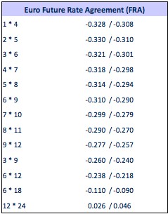
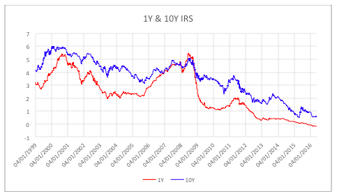
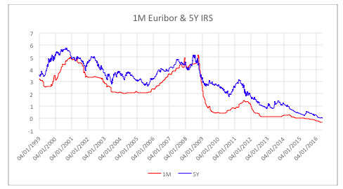
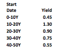
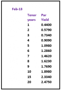
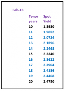
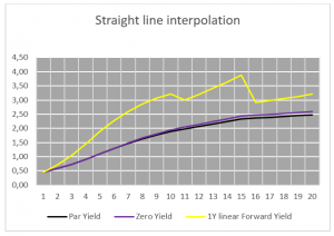
A normal yield curve is usually upward sloping with diminishing increases in yield– the longer the tenor, the higher the interest rate. Generally it is assumed that longer maturities contain larger risks for lenders and they require adequate compensation with a risk premium in the form of a liquidity spread.

Any long-term corporate investment (purchasing of plant and/or equipment) will need to be financed.

Normally if an asset has a service life of 15 years a loan would be arranged whereby the tenor was also 15 years. Assuming straight line depreciation of the asset then the annual principal repayment would equal the annual depreciation in the bookkeeping. So whilst we could then conclude that the ultimate tenor of a loan should equal the service life of an asset, it still does not answer how we should finance it.

Since January 1999, with the introduction of the Euro, it has become easier to collate data relating to interest rates on a daily basis. On the basis of working days (so days where rates will be traded and then published) there have been over 4,400 dates from which data could be collected. A daily array of interest rates both short and long term implies that it is not inconceivable that more than 75,000 individual data points could have been collated by now – perhaps a lot more depending on your appetite for data. It would be fair to say that this would represent a substantial array of data that could be analyzed.

Let us make the following assumptions:

  • We have access to this data
  • It contains all Euribor rates
  • It contains long term interest rate swap rates
  • We wish to compare long term fixed funding with short term funding
  • Short term funding is not only against Euribor but also shorter date long term swaps that have a maturity smaller than the long term fixed funding period
  • All trades can take place at the rates that we have captured and collated
  • The long term maturity is a fixed number of whole years
  • The short dated long term swaps are also a fixed number of whole years
  • We ignore the NPV of the cash flows
  • The short dated long term swaps are factors of the long term maturity
  • Interest payments on all interest rate swaps is annually

If we were to analyse 10 year fixed rates against shorter dated rollover funding we can compare it against periods of 1, 3 and 6 months as well as 1, 2 and 5 years.

The following is an analysis of data from the 4th of January 1999 up to and including the 31st May 2016.

Schermafbeelding 2016-06-30 om 10.12.18

Observations:

  • This overview is compiled as of the 31st May 2016.
  • If we look at 10Y (fixed) versus 1Y (fixed) rollover we see there are 1,925 data points.
  • If we look at 10Y (fixed) versus 5Y (fixed) rollover we see there are 3,183 data points.
  • The last date that we can calculate for 10Y against 1Y is 9 years before the 31st May 2016 – 31/05/2007
  • The last date that we can calculate for 10Y against 5Y is 5 years before the 31st May 2016 – 31/05/2011

Whilst interest rates have fallen since the crisis that started in the summer of 2008, rates were “normal” for the preceding 9 ½ years since the inception of the Euro in 1999.

Here is a graph of 1Y and 10Y IRS rates since 1999 –

Schermafbeelding 2016-06-30 om 10.14.38

As is to be expected the 10 year yield is normally higher than the 1 year yield – this follows the accepted theory for interest rates.

For further analysis here is a graph of 1Month Euribor and 5Y IRS rates since 1999 –

Schermafbeelding 2016-06-30 om 10.16.06

Yet again, as expected, the 5 year yield is normally higher than the 1 month yield.

So whilst the data produces normal curves whose general shape and distribution meet the expected theories of interest rates, regardless of the absolute value at any particular time, the analysis of the data shows that, in most cases fixing rates for a shorter term leads to lower interest charges than immediately fixing for a longer period.

Naturally, with the extremely low interest rates that are prevalent at the moment, it would be very naïve to conclude that interest rates should always be fixed for a shorter term than the desired tenor for the longer term. However, as mentioned in one of my previous articles about implied forwards,  it is necessary to look at all the implied values within a curve at the time that a loan needs to be arranged.

A quick and dirty inspection of the yield curve at the moment would show that, if we were looking at a constant 10 year yield curve priced off IRS, the implied curve would look like this at certain points –

Schermafbeelding 2016-06-30 om 10.22.19

Now we need to quantify the savings that, theoretically, could have been obtained by looking  at our original data.

Schermafbeelding 2016-06-30 om 10.18.29

As can be seen, a 5 year rollover fixed at inception and then refixed after 5 years as opposed to a 10 year fixed at inception led to an average reduction in interest costs of 122 basis points per annum and would have been the better option in 98.7% of the time.

There are no guarantees about prices in the future, but a lot more implied data is available in the current yield curve than just that one single curve that is shown as a graph in the newspapers.


Lionel Pavey


Lionel Pavey

Cash Management and Treasury Specialist – Flex Treasurer


Yield Curves (term structure of interest rates) – filling in the blanks

| 27-05-2016 | Lionel Pavey

Most treasurers do not have access to a dedicated financial data vendor (Bloomberg, Reuters) but are regularly faced with having to discover prices related to yield curves. There are websites that can provide us with relevant data, but these are normally a snapshot and not comprehensive – the data series is incomplete. It is therefore up to the treasurer to complete the series by filling in the blanks.

A quick refresher about the construction of a yield curve raises the following points:-

  • All data must be from the same market (treasury bonds, Interest Rate Swaps (IRS) etc.)
  • A regular term (maturity) is preferred for ease of construction
  • A curve must be smooth
  • An implied zero yield curve can be built from the smooth par curve – a theoretical yield curve where no interest is paid until maturity. In a bond this would redeem at par (100) and be issued at a deep discount to par
  • A series of discounted cash flow factors (DCF) are produced
  • An implied forward curve with constant maturities can be built from the par curve
  • An implied forward curve must be monotonic – each point in an increasing sequence is greater than or equal to the preceding point, each point in a decreasing sequence is smaller than or equal to the preceding point

If we look at IRS par yield prices that can be found on a website, we can regularly see yield prices for periods from 1 year to 10 year inclusive, a 15 year price and a 20 year price. To construct a complete curve from 1 year up to and including 20 years we need to fill in the blanks at 11,12,13,14,16,17,18 and 19 years. These yields are assumed to be par yields – the coupon rate is equal to the yield to maturity and the instrument trades at par.

Before starting let us define the procedure for constructing a par yield curve:-
The methodology used is called “bootstrapping”. This allows us to extract discount factors (DCF) from the market rates. DCF’s allow us to calculate a value today for a cash flow in the future.

We assume that the nominal value for all calculation purposes is 100

For a 1 year rate we know the interest and redemption amount at maturity. A DCF is built whereby the net present value (NPV) of these future cash flows in 1 years’ time is equal to 100 or par.

For a 2 year rate we receive interest after 1 year and interest and redemption amount at maturity.

We discount the 1st years’ interest with the DCF we obtained from the 1 year rate and deduct this amount from our initial nominal of 100. This net amount is then divided by the interest and redemption at maturity (at end of 2 years) to obtain the DCF for the 2 year rate.

Example:

1 Year                                      7%                          2 Year                          9%

1 Year      
100 / (7/100+100) = 0.93457944 (DCF)

2 Year
9 * 0.93457944 = 8.41121496
100 – 8.41121496 = 91.58878504
91.58878504 / (9/100+100) = 0.8402640829

These DCF’s can then be used to find the NPV of any cash flow maturing in 1 or 2 years’ time.

The following example shows a yield curve from February 2013 published on the website of an interbank broker.

yield curve February 2013

yield curve February 2013

The quickest way to price the missing periods would be with straight line interpolation of the par curve between the known points – which would produce the following par curve, zero yield curve and forward curve with constant 1 year maturity.

yield curve February 2013 - 2

yield curve February 2013

Straight line interpolation

Straight line interpolation


Whilst the par curve and zero curve are smooth, the implied 1 year constant maturity curve is jagged and certainly neither smooth nor monotonic. The 11th 1 year period rate is lower than the 10th period and the 15th 1 year period rate is higher than the 16th period.

A second approach would be to apply a weighting to the known periods of the par curve and to average the difference out over the missing periods. Read more on this second approach in my next article which will appear next week.

Lionel Pavey


Lionel Pavey

Treasurer