Lionel Pavey Archives - Page 6 of 7 - treasuryXL

How long can interest rates stay so low?

| 08-09-2016 | Lionel Pavey |

How long can interest rates stay so low? When we talk about interest rates, it is helpful if we know the basic theory of how the level of an interest rate is determined.Classical thinking states that there are 5 components in interest rates (x).

5 Components in interest rates:

Risk free rate – a constant rate with no inflation
Inflation – the future expectation for inflation is added to the risk free rate.
These, together, are called the nominal interest rate
Default risk premium – the individual credit score of the borrow
Liquidity premium – compensation for offering a product that can be difficult to sell on
Maturity premium – in a normal positive yield curve, longer maturities have a higher interest rate

A review of various data providers show that the “indicative rate” for a bullet loan with a maturity of 5 years for a Dutch local authority would be 0.06% per annum. Let us look as this rate compared to the 5 components already mentioned.

C, D and E are all premia and would, therefore, have a positive value. Even if their collective value was zero, it would imply that “nominal” 5 year interest rate would be 0.06%. This nominal rate, as previously stated, comprises both the risk free rate and the expected inflation.This leads to the presumption that either risk free rates are zero or that future expectations of inflation are negative.

According to the ECB inflation (HICP) index in July 2016 prices rose by 0.2% as an annual percentage change. The target inflation rate for the ECB is below, but close to, 2% over the medium term. Central banks set interest rates whilst keeping a watchful eye on headline and expected future inflation (it is a lagging indicator). Many studies claim that inflation indices overstate the true inflation figure, which would imply that the true inflation change would be zero or slightly negative.

If we were to enter a recession now there would be no room to use monetary policy as done previously as there is no space to lower rates any further. This would then only leave fiscal policy, but there is no unity within the Euro zone on fiscal policy.

It would appear that the present policy of quantitive easing (QE) has lead us to very low interest rates coupled with minimal inflation and no significant growth in GDP. Therefore, it is not improbable to envisage the current period of very low interest rates being maintained for quite some time in the future.

Furthermore, when QE stops, the ECB will eventually have to sell the bonds they are holding. Such an action could, conceivably, lead to a large rise in interest rates causing disruptions in the economic cycle. In the current environment, monetary policy can not revive the economy.

Lionel Pavey

Cash Management and Treasury Specialist – Flex Treasurer

Why companies still use Excel

| 25-08-2016 | Lionel Pavey |

Do you still rely on spreadsheets in your daily treasury operations? We have read multiple articles on this subject lately and we decided to ask our community: Why do treasurers still rely on spreadsheets? Yesterday Jan Meulendijks gave us his opinion on the topic. Today expert Lionel Pavey talks about the benefits of using Excel in your company.

Why do companies use Excel?

Cost – it is part of the Microsoft Office Package; low maintenance costs

Use – everyone has some level of proficiency with Excel

Versatile – data can be customized to your own requirements

Simplicity – comes preloaded with over 400 different formulae, though far less than 100 are truly needed for Treasury purposes

Training – most people learn on the job, no need for expensive courses to help people use the software

Flexible – give the same data to different people and see how they uniquely extract the data they need to answer their queries

Compatibility – all relevant data that is present on standalone accounting software etc. can be exported into Excel and adjusted for individual purposes to achieve the desired results

Problems with Excel?

Ignorance – getting staff to comprehend the route from input to output

Errors – not incorporating checks and balances that can highlight discrepancies

Individualism – is the output only for your consumption or is it passed on down through the chain, enhanced and then passed on again?

Disarray – everyone applies different fonts, layouts, conditional formatting. Should be a company policy in place to determine how data is collated and presented

Uncertainty – why do people insist on hiding columns and rows?

Duplication – the same spreadsheet data is present on many PC’s at the same time with subtle but significant differences. Someone has to own the original document

Solutions?

Dedicated BI software – expensive, no value outside of the present company normally, requires regular maintenance, multiple departments have to sign off before it can even be implemented, constant reviews of whether the correct modules are present, system updates

Design Structure – implement a company policy clearly dictating how “shared” spreadsheets are to be designed.

Input Structure – agree who delivers what, to whom, when and in the agreed format

Share results – allow other people to see how their data has been incorporated into the final reports so they can appreciate the significance of their contribution

Ownership – define who owns what part of the process (their level of responsibility) and who owns the spreadsheet

Reports – ensure that the end users clearly define what they require at the start. 10 versions of a spreadsheet before they get what they wanted means they did not know what they wanted or did not communicate clearly

Conclusion

Excel is well known, robust, versatile and understood. For cash flow forecasting 4 or 5 secure “master” spreadsheets can allow for most situations – daily cash flow recording, future cash flow forecasting, agreed budget, capital expenditure plans, funding commitments. These have to be well protected and isolated on the hard drive. Everything is a trade off – nothing will give you 100 per cent accuracy. However, if you can relatively simply design the required spreadsheets then data is always up to date and available when needed. This covers the 80 per cent of the time maxim– the other 20 per cent you will have to work harder to achieve. Excel is not going away – every new versions even more functionality that allows us to achieve the required level of input more easily whilst ensuring that the output can be better analysed and interpreted.

Lionel Pavey

Cash Management and Treasury Specialist

The impact of negative interest rates

01-08-2016 | Lionel Pavey |

Articles in the press state that large commercial banks are considering charging their corporate clients negative interest rates on credit balances on their bank accounts. This presents us with certain problems – how will clients react?

Withdraw money – known as stuffing money under the mattress. This would present huge security issues on where the money could be safely kept, potential theft etc. Holding cash would give a return equal to zero, which would be greater than depositing it at a bank.

Hoarding – by withdrawing money from the banking system, banks themselves would have less money to lend and would force them to reduce their balance sheets. Conversely the idea would be that people would spend more money rather than save and, therefore, boost the economy. Would it work? We are seeing negative yields on high quality government bonds, for a variety of reasons, yet it appears that negative rates have not boosted spending or investment. The loosening of monetary policy does not appear to have removed market fears.

Disintermediation – banks fulfill a role as intermediar/middleman in the supply chain of finance. If money is withdrawn from the banking system it would be even harder for banks to provide finance to lenders. How could lenders then obtain the funding they require? Virtual marketplaces could be envisaged but there are so many security and safeguard issues that would need to be addressed before this could take place. Most companies can not borrow from capital markets – they rely on banks to provide their funding. Reductions in government bond yields to below zero do not lead to more funding being given to companies.

Worst case scenarios – companies will invest in technologies that are capital intensive leading, eventually, to a fall in the demand for labour. Pensioners who are dependent on interest income will be forced to reduce their consumption leading to a fall in demand. With safe yields being negative the search for yield could lead investors into riskier assets than they would normally consider.

A stamp on physical cash – this is an idea more than 100 years old proposed by Gesell to stop hoarding of cash. Bank notes would need to receive a stamp every month to be considered valid cash. These stamps would have to be purchased (a form of negative interest) and their purpose would be to erode the principle that money is a store of value and could be better used by being actively invested in the economy.

This all sounds very pessimistic, but there are potential gains from negative interest rates for companies.

It would encourage companies to pay their creditors more quickly and, in the process, receive discounts on their purchases outstanding if they pay early. Furthermore it would enable companies to truly examine their whole supply chain across all departments within a company and create a better understanding of the workflow processes concerning cash receipts and disbursements.

For those who like a more rogue approach, you could actually overpay your creditors and ask for a credit note. Now your creditor is funding your negative interest rate and if true economic theory principles are maintained – a fall in prices should follow negative interest rates – then, not only you would have handed over your negative interest rate exposure but you would also benefit from falling prices in the future on the outstanding credit notes with your creditors allowing you to make a relative saving on the future purchase price.

It is clear that steering interest rates will not sort out the economy – other steps outside of monetary policy will have to be taken to restore faith in the economy. But which steps will that be?

Lionel Pavey

Cash Management and Treasury Specialist

Uitgelicht: Tekort aan obligaties dreigt voor ECB

| 28-07-2016 | Simon Knappstein, Lionel Pavey, Pieter Jan van Krevel |

Vorige week verscheen op fd.nl een artikel waarin wordt gesteld dat De Europese Centrale Bank in de knel dreigt te komen met haar grootschalige opkoopprogramma. Doordat de rente blijft dalen komen steeds minder staatsleningen in aanmerking voor opkoping. Wat heeft dit voor gevolgen? Wij vroegen experts Simon Knappstein, Lionel Pavey en Pieter Jan van Krevel om een reactie:

Simon Knappstein – Owner of FX Prospect

Dat er een tekort aan opkoopbare obligaties dreigt voor de ECB is sec geen probleem. Zij kunnen de regels zodanig aanpassen dat er meer obligaties in aanmerking komen. Alleen de keuze die ze maken kan sterke gevolgen hebben voor de banken en/of belastingbetaler.
Als de ECB de ondergrens van het opkoopprogramma verlaagt gelijk met de deposito rente dan komt er nog wat meer pijn bij de banken te liggen, en m.n. veel Italiaanse banken bevinden zich al in zwaar weer. Als de ECB alleen de ondergrens verlaagt lopen er meer kosten via de ECB, ergo de Europese belastingbetaler.
O.a. via de LTRO’s en TLTRO’s is er door de ECB al behoorlijke steun verleend aan de banken de afgelopen jaren, ik denk dat de ECB zal vinden dat het probleem van de Italiaanse banken lokaal fiscaal opgelost dient te worden.

Lionel Pavey – Cash Management and Treasury Specialist

No more bonds to buy? It appears that the ECB is running out of eligible bonds to purchase for its quantitive easing programme.
There are strict criteria to determine eligibility: no more than 33% of an issue can be purchased, bonds may not yield less than -0.4%, bond purchases per country are relative to the size of their economy – not the size of their outstanding debt.
Possible solutions:

Lower the interest rate criteria of -0.4%. More short dated bonds could be purchased.
Change the country criteria so that they are relative to the amount of outstanding debt – Italians would like that.
Start purchasing more long dated bonds (30 years) – would leave to a more pronounced flattening of the yield curve.

Problems:

QE was designed to stimulate the growth of inflation in the EU – this has failed.
EU rules state that the ECB are prohibited from directly buying government bonds as this would remove the motivation within a country to make their economies more competitive and reduce the pressure to rein in government overspending.
Inflation expectations are actually falling – bond yields are falling although this is also, but not solely, due to the QE.
The extra liquidity reaching banking system is not being shown in lending figures to corporates.
The economy of EU countries are not seeing rising GDP and falling unemployment.

The programme is not working. It is having a detrimental effect on interest rates that are constantly going down. Interest rates represent compensation for risk taken – so what does that make negative interest rates? 1 trillion Euros of debt have been purchased so far and no direct benefit has been seen in the economy. Time for a rethink and to blow the dust off our old economic textbooks to find a different solution.

Pieter Jan van Krevel – Owner of Slàinte Mhath!

Damned if you do. Damned if you don’t.
Het aantal kwalificerende staatsobligaties voor het ECB opkoopprogramma raakt langzamerhand uitgeput. Het verzwakken van de oorspronkelijke eisen van het programma zal uitdagingen produceren die zullen wedijveren met het verlies van vertrouwen dat de ECB lijdt bij het niet halen van haar ambitie EUR 80 mrd per maand op te kopen.
De meest logische stap lijkt het uitbreiden van het opkopen van bedrijfsobligaties in de Eurozone: tot dusverre is dit een onderdeel van het opkoopprogramma waar slechts in relatief beperkte mate invulling aan is gegeven, en uitbreiding hiervan dient in theorie nog directer de doelstelling van stimuleren van de economische groei en het aanwakkeren van de inflatie in de Eurozone.
De grootste uitdaging van de ECB op het vlak van de bedrijfsobligaties zal echter de breedte en diepte van de markt zijn, alsmede analyse van de kredietwaardigheid van de uitgevende bedrijven. De ECB als concurrent van S&P, Moody’s en Fitch…

How long should I fix an interest rate?

| 04-07-2016 | Lionel Pavey |

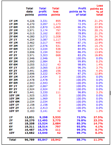
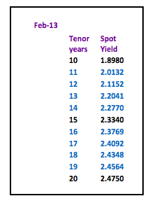
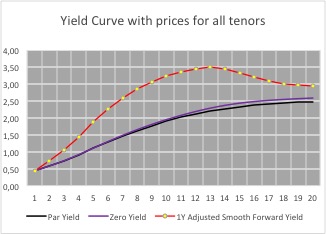
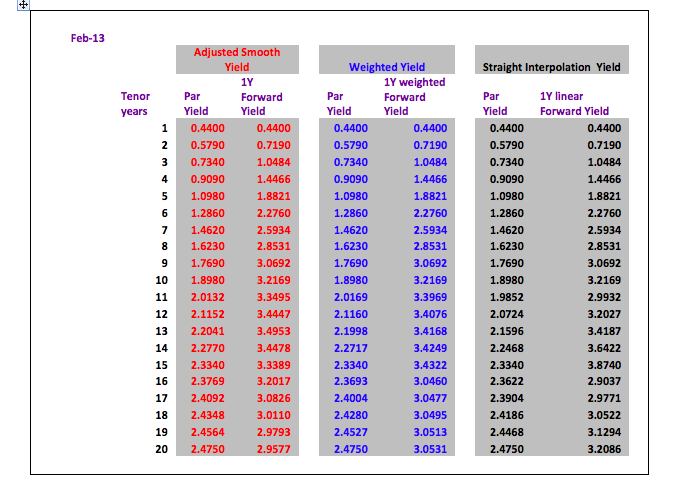
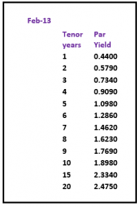
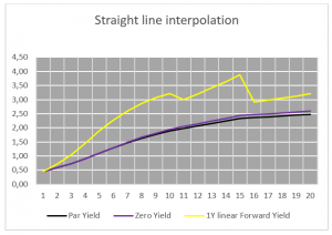
A normal yield curve is usually upward sloping with diminishing increases in yield– the longer the tenor, the higher the interest rate. Generally it is assumed that longer maturities contain larger risks for lenders and they require adequate compensation with a risk premium in the form of a liquidity spread.

Any long-term corporate investment (purchasing of plant and/or equipment) will need to be financed.

Normally if an asset has a service life of 15 years a loan would be arranged whereby the tenor was also 15 years. Assuming straight line depreciation of the asset then the annual principal repayment would equal the annual depreciation in the bookkeeping. So whilst we could then conclude that the ultimate tenor of a loan should equal the service life of an asset, it still does not answer how we should finance it.

Since January 1999, with the introduction of the Euro, it has become easier to collate data relating to interest rates on a daily basis. On the basis of working days (so days where rates will be traded and then published) there have been over 4,400 dates from which data could be collected. A daily array of interest rates both short and long term implies that it is not inconceivable that more than 75,000 individual data points could have been collated by now – perhaps a lot more depending on your appetite for data. It would be fair to say that this would represent a substantial array of data that could be analyzed.

Let us make the following assumptions:

We have access to this data
It contains all Euribor rates
It contains long term interest rate swap rates
We wish to compare long term fixed funding with short term funding
Short term funding is not only against Euribor but also shorter date long term swaps that have a maturity smaller than the long term fixed funding period
All trades can take place at the rates that we have captured and collated
The long term maturity is a fixed number of whole years
The short dated long term swaps are also a fixed number of whole years
We ignore the NPV of the cash flows
The short dated long term swaps are factors of the long term maturity
Interest payments on all interest rate swaps is annually

If we were to analyse 10 year fixed rates against shorter dated rollover funding we can compare it against periods of 1, 3 and 6 months as well as 1, 2 and 5 years.

The following is an analysis of data from the 4th of January 1999 up to and including the 31st May 2016.

Observations:

This overview is compiled as of the 31st May 2016.
If we look at 10Y (fixed) versus 1Y (fixed) rollover we see there are 1,925 data points.
If we look at 10Y (fixed) versus 5Y (fixed) rollover we see there are 3,183 data points.
The last date that we can calculate for 10Y against 1Y is 9 years before the 31st May 2016 – 31/05/2007
The last date that we can calculate for 10Y against 5Y is 5 years before the 31st May 2016 – 31/05/2011

Whilst interest rates have fallen since the crisis that started in the summer of 2008, rates were “normal” for the preceding 9 ½ years since the inception of the Euro in 1999.

Here is a graph of 1Y and 10Y IRS rates since 1999 –

As is to be expected the 10 year yield is normally higher than the 1 year yield – this follows the accepted theory for interest rates.

For further analysis here is a graph of 1Month Euribor and 5Y IRS rates since 1999 –

Yet again, as expected, the 5 year yield is normally higher than the 1 month yield.

So whilst the data produces normal curves whose general shape and distribution meet the expected theories of interest rates, regardless of the absolute value at any particular time, the analysis of the data shows that, in most cases fixing rates for a shorter term leads to lower interest charges than immediately fixing for a longer period.

Naturally, with the extremely low interest rates that are prevalent at the moment, it would be very naïve to conclude that interest rates should always be fixed for a shorter term than the desired tenor for the longer term. However, as mentioned in one of my previous articles about implied forwards, it is necessary to look at all the implied values within a curve at the time that a loan needs to be arranged.

A quick and dirty inspection of the yield curve at the moment would show that, if we were looking at a constant 10 year yield curve priced off IRS, the implied curve would look like this at certain points –

Now we need to quantify the savings that, theoretically, could have been obtained by looking at our original data.

As can be seen, a 5 year rollover fixed at inception and then refixed after 5 years as opposed to a 10 year fixed at inception led to an average reduction in interest costs of 122 basis points per annum and would have been the better option in 98.7% of the time.

There are no guarantees about prices in the future, but a lot more implied data is available in the current yield curve than just that one single curve that is shown as a graph in the newspapers.

Lionel Pavey

Cash Management and Treasury Specialist – Flex Treasurer

Constructing a yield curve for local authority loans

| 22-06-2016 | Lionel Pavey |

So far in this series we have constructed yield curves based on Interest Rate Swaps. This route was chosen as Swaps provide the benchmark for pricing many loan products. Let us look at constructing a yield curve for local authority loans. Yet again, the choice has been made for a product where prices are published on a daily basis.

The data that is published is not as comprehensive as that for Swaps but, using the procedures shown before, we are still able to build a curve. Only 3 data points were published – 1 year, 5 year and 10 year. It is thus possible to build a 10 year curve – the data is as follows:

Going back to the principles employed when building the IRS curve we shall make a first attempt by using linear interpolation of the spreads – a reasonably obvious approach. I shall save you all the calculations and simply say that this approach leads to an implied 1 year constant maturity curve that is not completely smooth – there is a peak in the period starting in 4 years.

Obviously you could manually alter the prices to achieve a better curve or make use of a curve building model like Nelson & Siegel. Personal experience has resulted in my preference being to calculate the ratio between the local authority rates and the swap rates and allowing the model to find a best fit. Ratios are generally less volatile than the input rates allowing for a better fit. Eventually an implied local authority curve can be built as shown below:

As previously shown the spread is also monotonic – constantly rising. Consider the implications if we know that a 10 year loan has a spread of 70 basis points over swaps whilst the 1 year loan has a spread of only 2 basis points over swaps.

A 10 year spread can also be defined as the weighted average of all the underlying 1 year constant maturities, so let us investigate how this works in this model:

A 10 year spread of 70 basis points starts with a spread of 2 basis points in the 1^st year rising in the 10^th year to 131 basis points when compared to the underlying implied 1 year constant swap curve. As a treasurer it is important to know how rates are constructed and determine for yourself what the best approach is to your funding needs. Where do you think rates will be in the future, what will the spreads be, borrow for 10 years or borrow for 5 years and renegotiate? A fixed spread is therefore very advantageous for the lender.

No one knows the future but the ability to calculate the implied future price can assist in making decisions now regarding the future. Long dated fixed loans are difficult to break open leading to potential opportunity losses. Bullet loans are the easiest to price, but by focusing only on the cash flows and not their individual time buckets it is possible that the best decisions are not always made. Linear loans are less transparent when pricing but, yet again, a different time approach can be used to make the process simpler. Rollercoaster loans used in construction and infrastructure projects are the most opaque but can also be viewed in a different light if approached in another manner.

Next – Opportunity loss/profit. If I could turn back time or see into the future

Lionel Pavey

Cash Management and Treasury Specialist – Flex Treasurer

Lionel Pavey about the German Bund Yield. Is there a solution?

| 17-06-2016 | Lionel Pavey |

This week’s headlines were all about the German Bund Yield hitting a historic low. On Wednesday we also published an article about this subject and asked our experts to respond. Expert Lionel Pavey reacts with a full article on the German Bund Yield and asks himself; is there a solution?

Possible reasons:

Flight to quality – investors looking to place their money in a safe place
Brexit referendum – polls suggest chance of exit greater than ever leading to uncertainty
Quantitative easing – ECB policy of buying government bonds pushes bond prices up and decreases the yield

Since 2008 governments have attempted to kickstart their economies using monetary policy – lower rates and quantitative easing. The sellers of government bonds who receive cash do not appear to be either spending it or investing it – a report from Merrill Lynch states that fund managers are sitting on more cash than at any times since 2001 and have reduced their shareholdings to their lowest level in 4 years.

It would appear that all efforts by central banks via monetary policy have not succeeded. If government yield are persistently negative there is a possibility of stagflation and important investment decisions being deferred to a future date, leading to falling prices and a vicious downward spiral.

Is there a solution?

When I studied economics there were 2 schools of thought at the time – Milton Friedman and John Maynard Keynes. I have always felt that Keynes was discarded rather harshly by the monetarists.

Keynes stated that in recessions the aggregate demand of economies falls. In other words, businesses and people tighten their belts and spend less money. Lower spending results in demand falling further and a vicious circle ensues of job losses and further falls in spending. Keynes’s solution to the problem was that governments should borrow money and boost demand by pushing the money into the economy. Once the economy recovered, and was expanding again, governments should pay back the loans.

It is that last sentence that is pertinent. Keynes’ remedy runs countercyclical to the business cycle –instead of using all the money to buy up Government Debt, Government should borrow the money directly and embark on large projects to improve the infrastructure within a country. When the economy was revived Government should then repay the money borrowed and run a budget surplus.

Lionel Pavey

Cash Management and Treasury Specialist – Flex Treasurer

Talk of the day: German Bund Yield Below 0%

| 15-06-2016 | Udo Rademakers, Rob Söentken, Douwe Dijkstra & Lionel Pavey |

For the first time ever the German bund yield hit negative territory. The ‘Deutsche Welle’ writes: “With the prospect of Britain leaving the European Union looming ever larger ahead of referendum in 9 days, global investors are increasingly fleeing to safe havens such as German debt and Japenese currency. As a result, the yield on Germany’s benchmark 10-year debt fell into negative territory for the first time in its history on Tuesday. ” (DW.com) We asked some of our experts to give their opinion on this news:

Udo Rademakers
“Billions of Euro´s are invested into sovereign debt, even if meanwhile investors need to pay for this. German yield prices can meanwhile compete with Japan and Swiss rates (all below 0). The mainstream media explains this development as “concerns about the economic and political risks of a Brexit” and “concerns about the state of global growth”. However, the longer term trend since the 1980´s has been downwards and we now see a kind of (last?) acceleration in price.

Knowing the challenges Europe (and Germany) is facing, I think it is a matter of time before we could expect a spike in the rates again….. .I would place my bet in other markets.

Every trend is coming to an end…….”

Rob Söentken
“Not even a month ago markets were discounting the impact of the Brexit referendum. Now in a matter of weeks the odds have swung back from around 25% in favor of leaving to 42%. The increased media attention and figures (true or false) being thrown around are making voters run to register to vote. Apparently it’s mostly younger voters, who tend to be more in favor of staying. It is said that a turnup above 60% is favorable to the ‘remain’ vote. Still both camps are becoming more and more committed.

The downside for GBP vs EUR is probably the biggest risk. If the UK leaves the EUR, UK equities may dip sharply, but will likely recover because of the prospect of more independent monetary and economic policy. Interest rates will probably start rising to incorporate the increased independence risks. But the GBP as a currency may dip an absolute 10% or more, anticipating asset sales from foreign investors. Investors will fear the UK will become like Italy and France in the past: a country that needs to devalue its currency on a regular basis to offset internal rigidities and inefficiencies.”

Douwe Dijkstra
“Who would have thought this a few years ago, the interest rate on 10- year German government bonds below zero percent. For some time we hear our banks and advisors recommending to fix our interest rate exposure because its “now or never”.

However, anyone who has fixed already acted too early. For one of my clients I’m busy to Blend & Extend their current IRS contracts, fixing the interest rate for 7 years. Afterwards too early? Nobody knows. I think my client will have no regrets rather ” sooner than later”!”

Lionel Pavey

“Possible reasons:

Flight to quality – investors looking to place their money in a safe place
Brexit referendum – polls suggest chance of exit greater than ever leading to uncertainty
Quantitative easing – ECB policy of buying government bonds pushes bond prices up and decreases the yield

More on this topic in my article which will be published on Friday.”

What’s your opinion on this news? Let us know in the comment section below.

Zero Coupon Yields and implied Forward Yields

| 13-06-2016 | Lionel Pavey |

Having constructed our 20 year yield curve with both observable data and discovered data in my previous article,we are now in possession of 3 sets of data:

Spot par rates
Spot zero coupon rates
Discounted Cash Flow factors (DCF)

The most important of these, for calculation purposes, is DCF.

Present Value

The discounted present value of a future cash flow can be calculated by dividing the future value by the DCF. It therefore follows that a series of future cash flows can also be discounted to a single net present value.

Implied Forward Rates

The original yield curve showed annual spot rates for a period of 20 years. Using DCF it is possible to construct similar curves but with forward start dates – a curve starting in 1 year, 2 years, 3 years etc. When building these curves the “implied” forward rate will actually be a zero coupon rate and not a par rate. Converting the zero rates to par rates can be achieved by using Excel Solver – a very useful tool but great care must be taken as Solver gives an answer but shows no formula.

So, how do we calculate an implied forward rate?

Let us assume that we wished to find a rate with a duration of 4 years, starting 5 years forward.
To achieve that, we need both the 5 year DCF and the 9 year DCF

The previous constructed curve yields the following values –

5Y DCF = 0.9464924176

9Y DCF = 0.8508986778

((.9464924176/.8508986778)^(1/4)-1)*100 = 2.6975% implied 4 year rate starting in 5 years

As stated, this is the implied zero coupon rate – the implied par rate is 2.6887%

All forward rates are purely implied rates – a true quoted rate would always be different for various reasons –

Spread between bid and offer
Yield curve constructed with specific data
Sentiment of the trader
Possible exposure already in the banks’ books

Here is a small snapshot of both implied rates and par rates built with the original curve.

When I discussed building the original yield curve, different ways of interpolation were tried. I would now like to show how small differences in yields in a spot curve can lead to significant differences in a forward curve.

Let us look at a duration of 5 years starting 10 years in the future and compare the linear interpolation with the smooth adjusted curve. Assume that the instrument to be priced is a linear instrument – equal repayments of principal every year.

I have built both curves using the same layout and formulae throughout with the exception of the input rates in the missing periods.

The linear rate is 3.276%; the smooth adjusted rate is 3.416% – a difference of 14 basis points or about 4% of the smooth rate. In a market where the normal bid/offer spread is about 3 or 4 basis point, this represents a significant difference/anomaly.

I regularly hear people say that when they need to purchase a financial instrument that they get at least 2 quotes – this is all very well but does not stop a treasurer from first ascertaining what the correct price should be before getting a quote. If banks know that, as a treasurer, you can not calculate the theoretical price this allows them to move the price away from the implied to a price that is more advantageous to them and their trading book! A dedicated financial data vendor system can make life easier, but it is not impossible to calculate a price without these resources!

Next – Spreads; their use and the hidden extra costs

First two articles on building a yield curve:
1. Yield Curves (term structure of interest rates) – filling in the blanks
2. Yield Curves (term structure of interest rates) – filling in the blanks part II

Lionel Pavey

Treasurer

Yield Curves (term structure of interest rates) – filling in the blanks part II

| 03-06-2016 | Lionel Pavey |

Most treasurers do not have access to a dedicated financial data vendor (Bloomberg, Reuters) but are regularly faced with having to discover prices related to yield curves. There are websites that can provide us with relevant data, but these are normally a snapshot and not comprehensive – the data series is incomplete. It is therefore up to the treasurer to complete the series by filling in the blanks. In my previous article I went over the first approach. Today I’ll talk about the second approach.

A second approach would be to apply a weighting to the known periods of the par curve and to average the difference out over the missing periods.

This leads to 1 year constant maturity rates that are almost equal in value for all the periods between 2 known periods. Whilst these forward rates are also not correct they at least supply us with a visual indicator as to the general shape of the forward yield curve – the 1 year constant maturity rates

reach their zenith between years 12 and 14; after that point they then start to decrease.

Futhermore, taking into consideration the yield curve as shown in the graph, we can make the following conclusions about the 1 year curve:-

11 year rate must be higher than the linear interpolated rate but lower than the weighted interpolated rate
13 year rate must be higher than the weighted interpolated rate
15 year rate must be lower than the linear interpolated rate and lower than the weighted interpolated rate
16 year rate must be higher than the linear interpolated rate and higher than the weighted interpolated rate
20 year rate must be lower than the linear interpolated rate and lower than the weighted interpolated rate
The implied forward 1 year constant maturity curve must be smooth and monotonic.

On the basis of these restraints a par curve can be built that leads to the following forward curve.

The rates for the missing periods have been calculated manually whilst adhering to the conditions mentioned before– there are formulae which would allow rates to be discovered (Cubic spline, Nelson Siegel etc.) – but these rely on random variables and I have yet to see anyone quote and trade prices based solely on a mathematical formulae.

Visually, the 1 year curve meets all the criteria for the construction of a yield curve, together with the underlying par and zero yield curves.

To ascertain that the rates are correct, discount all the cash flows of the par yield for the given maturity – they should equal 100.

Here is an overview of all the implied 1 year rates using the different methods to construct the yield curve.

Conclusion:

For a quick calculation a straight line interpolation is acceptable with the warning that with a normal positive yield curve the real prices will be higher than the prices calculated by straight line interpolation. For a negative yield curve this would be reversed – real prices lower than interpolated prices.

The average difference between the par yield prices of the adjusted smooth yield and the straight interpolation yield are only 2.5 basis points. However, this difference is magnified when looking at a 1 year forward yield curve where the average difference is 22.5 basis points per period with a maximum of 53.5 basis points.

Next – Zero Coupon Yields and implied Forward Yields

Would you like to read part one of this article?
– Yield Curves (term structure of interest rates) – filling in the blanks

Lionel Pavey

Treasurer

How long can interest rates stay so low?

5 Components in interest rates:

Why companies still use Excel

Why do companies use Excel?

Problems with Excel?

Solutions?

Conclusion

The impact of negative interest rates

Uitgelicht: Tekort aan obligaties dreigt voor ECB

How long should I fix an interest rate?

Constructing a yield curve for local authority loans

Lionel Pavey about the German Bund Yield. Is there a solution?

Possible reasons:

Is there a solution?

Talk of the day: German Bund Yield Below 0%

Zero Coupon Yields and implied Forward Yields

Present Value

Implied Forward Rates

Yield Curves (term structure of interest rates) – filling in the blanks part II

Conclusion:

Go to

Partner Program

Contact us

Subscribe